State-Level Fertility Distributions

workflowr

• Summary
• Checks
• Past versions

Last updated: 2026-04-24

Checks: 6 1

Knit directory: USC-QCB-IPUMS/

This reproducible R Markdown analysis was created with workflowr (version 1.7.1). The Checks tab describes the reproducibility checks that were applied when the results were created. The Past versions tab lists the development history.

---

R Markdown file: up-to-date

Great! Since the R Markdown file has been committed to the Git repository, you know the exact version of the code that produced these results.

Environment: empty

Great job! The global environment was empty. Objects defined in the global environment can affect the analysis in your R Markdown file in unknown ways. For reproduciblity it’s best to always run the code in an empty environment.

Seed: set.seed(20230130)

The command set.seed(20230130) was run prior to running the code in the R Markdown file. Setting a seed ensures that any results that rely on randomness, e.g. subsampling or permutations, are reproducible.

Session information: recorded

Great job! Recording the operating system, R version, and package versions is critical for reproducibility.

Cache: detected

The following chunks had caches available:

• load-data

To ensure reproducibility of the results, delete the cache directory state_fertility_cache and re-run the analysis. To have workflowr automatically delete the cache directory prior to building the file, set delete_cache = TRUE when running wflow_build() or wflow_publish().

File paths: relative

Great job! Using relative paths to the files within your workflowr project makes it easier to run your code on other machines.

Repository version: 5634d2b

Great! You are using Git for version control. Tracking code development and connecting the code version to the results is critical for reproducibility.

The results in this page were generated with repository version 5634d2b. See the Past versions tab to see a history of the changes made to the R Markdown and HTML files.

Note that you need to be careful to ensure that all relevant files for the analysis have been committed to Git prior to generating the results (you can use wflow_publish or wflow_git_commit). workflowr only checks the R Markdown file, but you know if there are other scripts or data files that it depends on. Below is the status of the Git repository when the results were generated:

Ignored files:
    Ignored:    .DS_Store
    Ignored:    .Rhistory
    Ignored:    .Rproj.user/
    Ignored:    analysis/hunt_paper2_figures_cache/
    Ignored:    analysis/state_fertility_cache/

Untracked files:
    Untracked:  Rplots.pdf
    Untracked:  analysis/hunt_paper2_figures.Rmd

Unstaged changes:
    Modified:   .claude/settings.local.json

Note that any generated files, e.g. HTML, png, CSS, etc., are not included in this status report because it is ok for generated content to have uncommitted changes.

---

These are the previous versions of the repository in which changes were made to the R Markdown (analysis/state_fertility.Rmd) and HTML (docs/state_fertility.html) files. If you’ve configured a remote Git repository (see ?wflow_git_remote), click on the hyperlinks in the table below to view the files as they were in that past version.

File	Version	Author	Date	Message
Rmd	5634d2b	Tina Lasisi	2026-04-16	updated plots
html	5634d2b	Tina Lasisi	2026-04-16	updated plots
Rmd	61c2f18	Tina Lasisi	2026-04-14	Update state_fertility.Rmd
html	027da76	Tina Lasisi	2026-04-14	updated figures
Rmd	71cf78a	Tina Lasisi	2026-04-14	updated figures
html	71cf78a	Tina Lasisi	2026-04-14	updated figures
Rmd	39a5a72	Tina Lasisi	2026-04-14	Update state_fertility.Rmd
html	34bd822	Tina Lasisi	2026-04-14	Update plots
Rmd	1439d7c	Tina Lasisi	2026-04-14	Update state_fertility.Rmd
Rmd	9ef76c8	Tina Lasisi	2026-04-14	Update state_fertility.Rmd
Rmd	9d44b29	Tina Lasisi	2026-04-14	updated figures etc
html	9d44b29	Tina Lasisi	2026-04-14	updated figures etc
Rmd	79eb4de	Tina Lasisi	2026-04-14	added birth cohort stability analysis
html	79eb4de	Tina Lasisi	2026-04-14	added birth cohort stability analysis
html	df537cf	Tina Lasisi	2026-04-14	Build site.
Rmd	bede61f	Tina Lasisi	2026-04-14	State by state figures added
html	bede61f	Tina Lasisi	2026-04-14	State by state figures added

---

Introduction

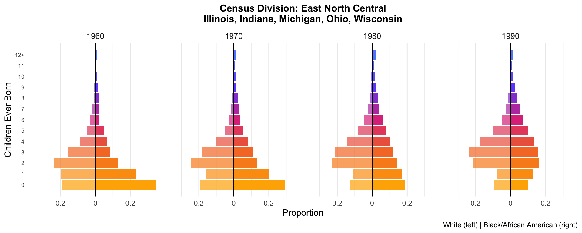
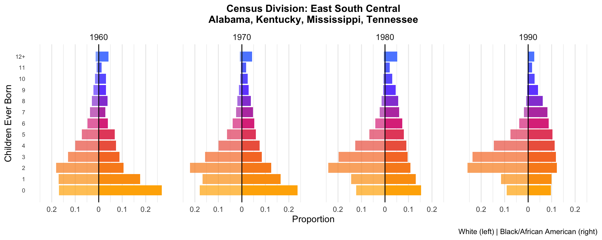
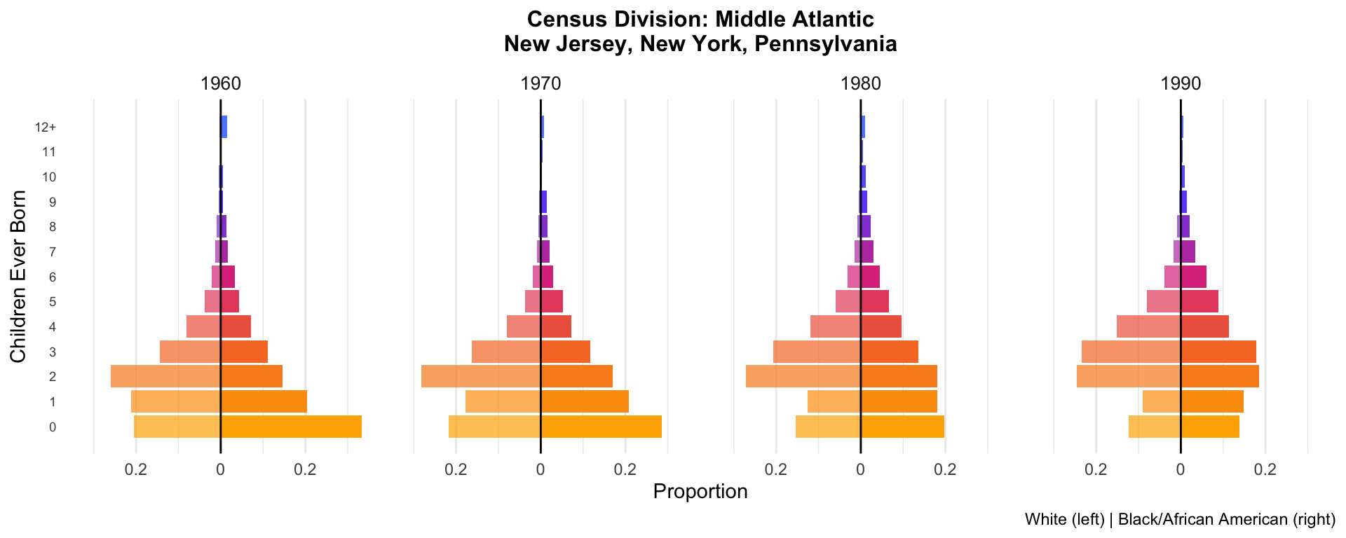
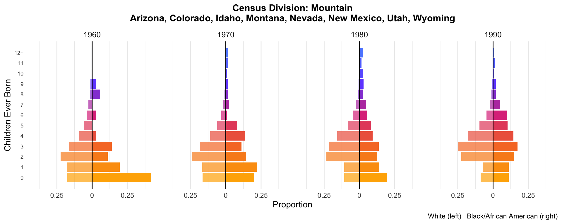
This analysis extends the national-level fertility distribution analysis to the state level, using IPUMS USA Census microdata (1960–1990, 1% samples). We produce choropleth maps of mean and variance in children ever born by state, race, and census year, followed by per-state mirrored bar charts for states with adequate sample sizes.

library(ipumsr)
library(tidyverse)
library(data.table)
library(usmap)
library(viridis)
library(patchwork)
library(scales)
library(ggrepel)

source("code/utils_fertility.R")

1. Load and process data

Update the DDI filename below to match your state-level extract (e.g., usa_00007.xml). Run code/get_state_extract.R first to download the extract.

# UPDATE this filename to match your downloaded extract
extract_name <- "usa_00007"

setwd("data")
ddi <- read_ipums_ddi(paste0(extract_name, ".xml"))
data_raw <- read_ipums_micro(ddi)

Use of data from IPUMS USA is subject to conditions including that users should cite the data appropriately. Use command `ipums_conditions()` for more details.

setwd("../")

cat("Raw data dimensions:", nrow(data_raw), "rows x", ncol(data_raw), "cols\n")

Raw data dimensions: 29704073 rows x 19 cols

data <- data_raw %>%
  prepare_ipums_labels() %>%
  filter_fertility_sample() %>%
  recode_chborn() %>%
  add_age_range() %>%
  filter(AGE_RANGE == "50-59")

# Cap children at 12 for display
data <- data %>%
  mutate(chborn_capped = pmin(chborn_num, 12))

# Extract state name from STATEFIP factor labels
data <- data %>%
  mutate(state_name = as.character(STATEFIP))

cat("Filtered data dimensions:", nrow(data), "rows\n")

Filtered data dimensions: 1405711 rows

cat("States:", n_distinct(data$state_name), "\n")

States: 51 

cat("Years:", sort(unique(data$YEAR)), "\n")

Years: 1960 1970 1980 1990 

2. Sample size diagnostics

With 1% samples, some state-race-year cells will have very few observations, especially for Black/African American populations in states with small minority populations. We flag cells with n < 30 and suppress those with n < 10.

cell_sizes <- data %>%
  count(state_name, RACE, YEAR, name = "n_obs") %>%
  mutate(
    flag = case_when(
      n_obs < 10  ~ "suppress",
      n_obs < 30  ~ "caution",
      TRUE        ~ "ok"
    )
  )

# Summary of flagged cells
cat("Cell size summary:\n")

Cell size summary:

cell_sizes %>%
  count(RACE, flag) %>%
  pivot_wider(names_from = flag, values_from = n, values_fill = 0) %>%
  print()

# A tibble: 2 × 4
  RACE                      ok caution suppress
  <fct>                  <int>   <int>    <int>
1 White                    204       0        0
2 Black/African American   141      17       29

cell_sizes %>%
  mutate(
    n_obs_log  = log10(n_obs + 1),
    text_color = if_else(n_obs_log < median(log10(n_obs + 1)), "white", "black")
  ) %>%
  ggplot(aes(x = as.factor(YEAR), y = reorder(state_name, state_name), fill = n_obs_log)) +
  geom_tile(color = "white", linewidth = 0.2) +
  facet_wrap(~ RACE) +
  scale_fill_viridis(option = "magma", name = "log10(n)") +
  scale_color_identity() +
  labs(
    title = "Sample Sizes by State, Race, and Census Year",
    subtitle = "Non-Hispanic women aged 40+, 1% samples",
    x = "Census Year",
    y = NULL
  ) +
  theme_minimal() +
  theme(
    axis.text.y = element_text(size = 6),
    strip.text = element_text(size = 11, face = "bold")
  )

Warning in mean.default(X[[i]], ...): argument is not numeric or logical:
returning NA
Warning in mean.default(X[[i]], ...): argument is not numeric or logical:
returning NA
Warning in mean.default(X[[i]], ...): argument is not numeric or logical:
returning NA
Warning in mean.default(X[[i]], ...): argument is not numeric or logical:
returning NA
Warning in mean.default(X[[i]], ...): argument is not numeric or logical:
returning NA
Warning in mean.default(X[[i]], ...): argument is not numeric or logical:
returning NA
Warning in mean.default(X[[i]], ...): argument is not numeric or logical:
returning NA
Warning in mean.default(X[[i]], ...): argument is not numeric or logical:
returning NA
Warning in mean.default(X[[i]], ...): argument is not numeric or logical:
returning NA
Warning in mean.default(X[[i]], ...): argument is not numeric or logical:
returning NA
Warning in mean.default(X[[i]], ...): argument is not numeric or logical:
returning NA
Warning in mean.default(X[[i]], ...): argument is not numeric or logical:
returning NA
Warning in mean.default(X[[i]], ...): argument is not numeric or logical:
returning NA
Warning in mean.default(X[[i]], ...): argument is not numeric or logical:
returning NA
Warning in mean.default(X[[i]], ...): argument is not numeric or logical:
returning NA
Warning in mean.default(X[[i]], ...): argument is not numeric or logical:
returning NA
Warning in mean.default(X[[i]], ...): argument is not numeric or logical:
returning NA
Warning in mean.default(X[[i]], ...): argument is not numeric or logical:
returning NA
Warning in mean.default(X[[i]], ...): argument is not numeric or logical:
returning NA
Warning in mean.default(X[[i]], ...): argument is not numeric or logical:
returning NA
Warning in mean.default(X[[i]], ...): argument is not numeric or logical:
returning NA
Warning in mean.default(X[[i]], ...): argument is not numeric or logical:
returning NA
Warning in mean.default(X[[i]], ...): argument is not numeric or logical:
returning NA
Warning in mean.default(X[[i]], ...): argument is not numeric or logical:
returning NA
Warning in mean.default(X[[i]], ...): argument is not numeric or logical:
returning NA
Warning in mean.default(X[[i]], ...): argument is not numeric or logical:
returning NA
Warning in mean.default(X[[i]], ...): argument is not numeric or logical:
returning NA
Warning in mean.default(X[[i]], ...): argument is not numeric or logical:
returning NA
Warning in mean.default(X[[i]], ...): argument is not numeric or logical:
returning NA
Warning in mean.default(X[[i]], ...): argument is not numeric or logical:
returning NA
Warning in mean.default(X[[i]], ...): argument is not numeric or logical:
returning NA
Warning in mean.default(X[[i]], ...): argument is not numeric or logical:
returning NA
Warning in mean.default(X[[i]], ...): argument is not numeric or logical:
returning NA
Warning in mean.default(X[[i]], ...): argument is not numeric or logical:
returning NA
Warning in mean.default(X[[i]], ...): argument is not numeric or logical:
returning NA
Warning in mean.default(X[[i]], ...): argument is not numeric or logical:
returning NA
Warning in mean.default(X[[i]], ...): argument is not numeric or logical:
returning NA
Warning in mean.default(X[[i]], ...): argument is not numeric or logical:
returning NA
Warning in mean.default(X[[i]], ...): argument is not numeric or logical:
returning NA
Warning in mean.default(X[[i]], ...): argument is not numeric or logical:
returning NA
Warning in mean.default(X[[i]], ...): argument is not numeric or logical:
returning NA
Warning in mean.default(X[[i]], ...): argument is not numeric or logical:
returning NA
Warning in mean.default(X[[i]], ...): argument is not numeric or logical:
returning NA
Warning in mean.default(X[[i]], ...): argument is not numeric or logical:
returning NA
Warning in mean.default(X[[i]], ...): argument is not numeric or logical:
returning NA
Warning in mean.default(X[[i]], ...): argument is not numeric or logical:
returning NA
Warning in mean.default(X[[i]], ...): argument is not numeric or logical:
returning NA
Warning in mean.default(X[[i]], ...): argument is not numeric or logical:
returning NA
Warning in mean.default(X[[i]], ...): argument is not numeric or logical:
returning NA
Warning in mean.default(X[[i]], ...): argument is not numeric or logical:
returning NA
Warning in mean.default(X[[i]], ...): argument is not numeric or logical:
returning NA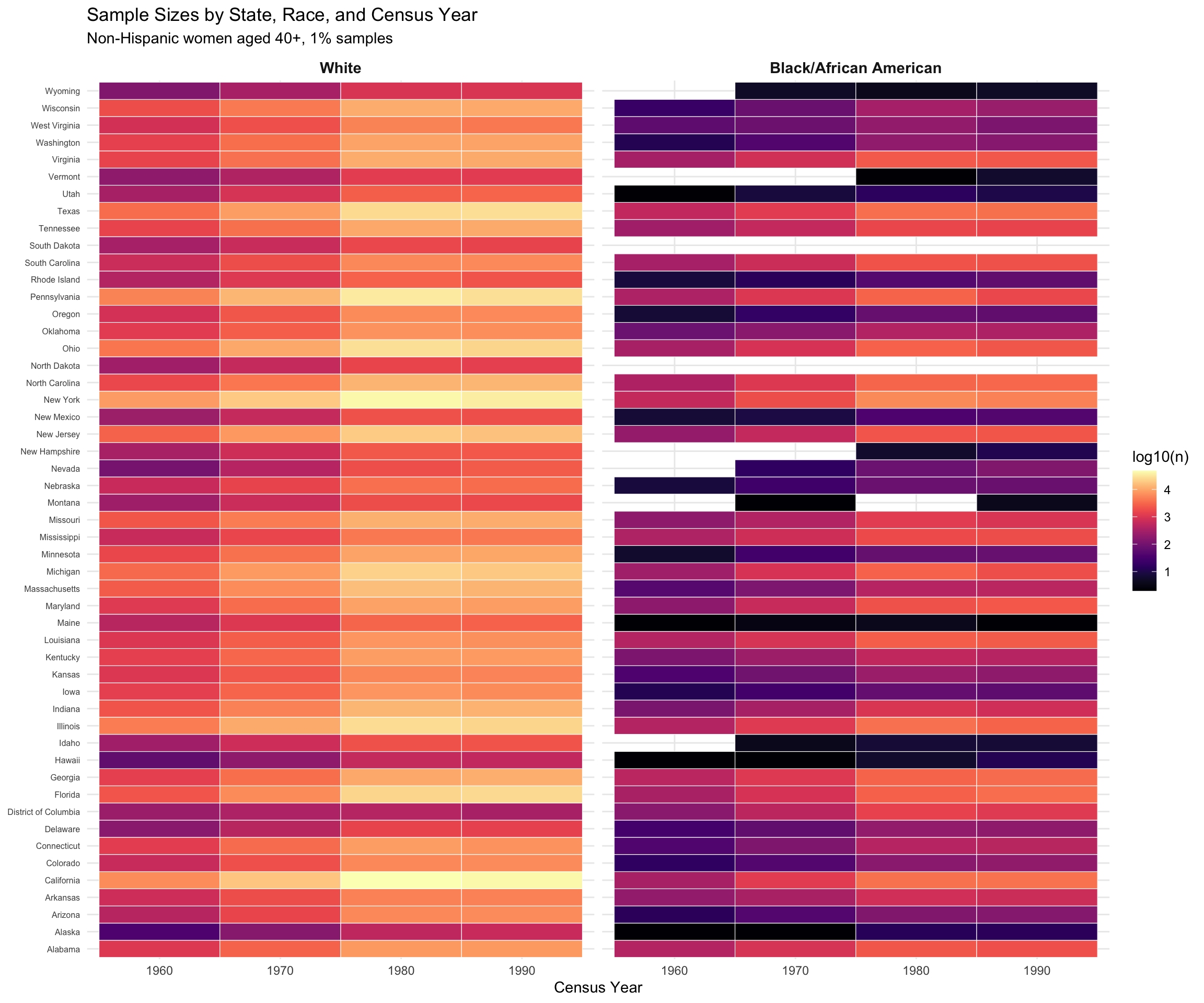

Past versions of sample-size-heatmap-1.png

Version	Author	Date
bede61f	Tina Lasisi	2026-04-14

3. State-level summary statistics

state_stats <- data %>%
  group_by(state_name, RACE, YEAR) %>%
  summarise(
    n_obs       = n(),
    mean_chborn = weighted.mean(chborn_num, w = PERWT),
    var_chborn  = sum(PERWT * (chborn_num - weighted.mean(chborn_num, w = PERWT))^2) / sum(PERWT),
    .groups = "drop"
  ) %>%
  # Suppress small cells
  mutate(
    mean_chborn = if_else(n_obs < 10, NA_real_, mean_chborn),
    var_chborn  = if_else(n_obs < 10, NA_real_, var_chborn)
  )

# Preview
state_stats %>%
  filter(state_name %in% c("California", "New York", "Mississippi", "Vermont")) %>%
  arrange(state_name, RACE, YEAR) %>%
  print(n = 40)

# A tibble: 30 × 6
   state_name  RACE                    YEAR n_obs mean_chborn var_chborn
   <chr>       <fct>                  <int> <int>       <dbl>      <dbl>
 1 California  White                   1960  6453        1.85       3.14
 2 California  White                   1970 17561        2.04       2.94
 3 California  White                   1980 47609        2.52       3.12
 4 California  White                   1990 41672        2.62       2.77
 5 California  Black/African American  1960   327        2.09       7.00
 6 California  Black/African American  1970  1149        2.36       6.90
 7 California  Black/African American  1980  3801        3.00       7.58
 8 California  Black/African American  1990  3898        3.33       5.82
 9 Mississippi White                   1960   644        3.02       6.54
10 Mississippi White                   1970  1515        2.56       4.53
11 Mississippi White                   1980  4400        2.78       3.88
12 Mississippi White                   1990  4376        2.83       2.89
13 Mississippi Black/African American  1960   378        3.46      12.5 
14 Mississippi Black/African American  1970   756        3.99      14.5 
15 Mississippi Black/African American  1980  1700        5.03      14.3 
16 Mississippi Black/African American  1990  1827        4.99      11.1 
17 New York    White                   1960  8287        1.95       3.16
18 New York    White                   1970 18882        1.98       2.97
19 New York    White                   1980 42030        2.47       3.47
20 New York    White                   1990 35522        2.68       3.38
21 New York    Black/African American  1960   600        1.87       4.86
22 New York    Black/African American  1970  1851        2.05       5.20
23 New York    Black/African American  1980  6089        2.63       6.38
24 New York    Black/African American  1990  5098        2.90       5.50
25 Vermont     White                   1960   184        2.69       7.13
26 Vermont     White                   1970   400        2.63       4.75
27 Vermont     White                   1980  1200        3.15       4.64
28 Vermont     White                   1990  1175        3.15       3.50
29 Vermont     Black/African American  1980     1       NA         NA   
30 Vermont     Black/African American  1990     5       NA         NA   

4. Choropleth maps: Mean children ever born

# usmap requires a 'fips' column or 'state' column
map_data_mean <- state_stats %>%
  rename(state = state_name)

plot_maps <- function(map_df, fill_var, title, caption = NULL, palette_option = "magma") {
  years <- sort(unique(map_df$YEAR))
  races <- c("White", "Black/African American")

  plots <- list()
  for (y in years) {
    for (r in races) {
      sub <- map_df %>% filter(RACE == r, YEAR == y)
      p <- plot_usmap(data = sub, values = fill_var, color = "grey70", linewidth = 0.2) +
        scale_fill_viridis(
          option = palette_option, na.value = "grey90",
          name = fill_var, limits = range(map_df[[fill_var]], na.rm = TRUE)
        ) +
        labs(title = paste(y, "-", r)) +
        theme(plot.title = element_text(size = 9, hjust = 0.5))
      plots <- c(plots, list(p))
    }
  }

  # columns = races (2), rows = years — landscape orientation
  wrap_plots(plots, ncol = length(races)) +
    plot_layout(guides = "collect") +
    plot_annotation(title = title, caption = caption) &
    theme(
      legend.position = "bottom",
      plot.title = element_text(size = 14, hjust = 0.5)
    )
}

plot_maps(map_data_mean, "mean_chborn",
          "Mean Children Ever Born by State, Race, and Census Year",
          caption = "Weighted mean of children ever born (CHBORN) among non-Hispanic White and Black/African American women aged 50–59. Rows = census year; columns = race group. Grey = insufficient data (n < 10). Source: IPUMS USA 1% samples.")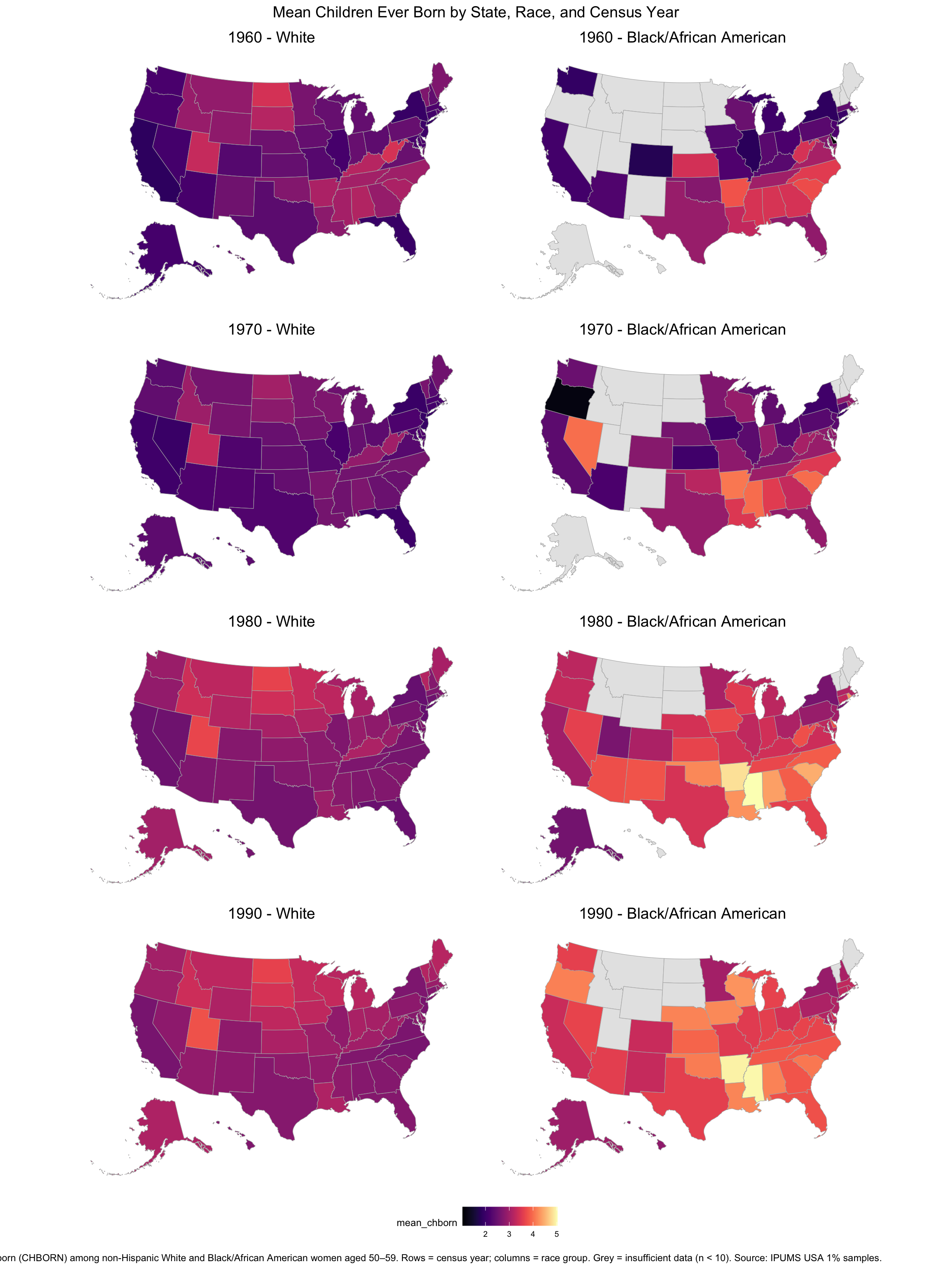

Past versions of map-mean-1.png

Version	Author	Date
71cf78a	Tina Lasisi	2026-04-14
bede61f	Tina Lasisi	2026-04-14

5. Choropleth maps: Variance in children ever born

plot_maps(map_data_mean, "var_chborn",
          "Variance in Children Ever Born by State, Race, and Census Year",
          caption = "Weighted variance of children ever born (CHBORN) among non-Hispanic White and Black/African American women aged 50–59. Higher values indicate greater spread in completed family sizes. Rows = census year; columns = race group. Grey = insufficient data (n < 10). Source: IPUMS USA 1% samples.",
          palette_option = "inferno")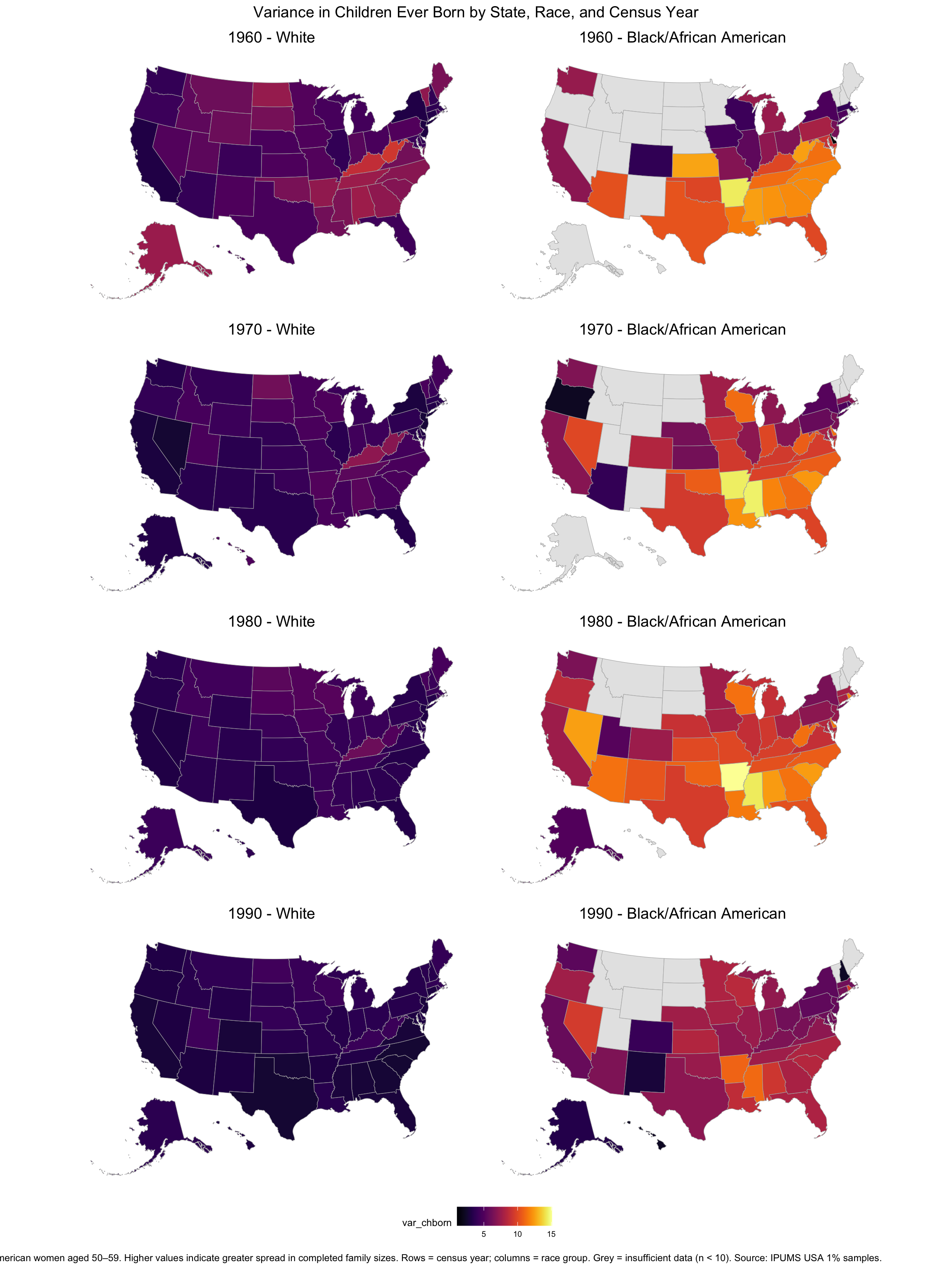

Past versions of map-variance-1.png

Version	Author	Date
71cf78a	Tina Lasisi	2026-04-14
bede61f	Tina Lasisi	2026-04-14

6. Choropleth maps: Zero inflation (proportion childless, age 50–59)

Women aged 50–59 have largely completed their fertility, making this age group a clean window onto childlessness patterns.

zero_inf_stats <- data %>%
  group_by(state_name, RACE, YEAR) %>%
  summarise(
    n_obs          = n(),
    n_zero_sample  = sum(chborn_num == 0),
    n_zero_pop     = sum(PERWT[chborn_num == 0]),
    n_total_pop    = sum(PERWT),
    prop_zero      = weighted.mean(chborn_num == 0, w = PERWT),
    .groups        = "drop"
  ) %>%
  mutate(across(c(n_zero_sample, n_zero_pop, n_total_pop, prop_zero),
                ~ if_else(n_obs < 10, NA_real_, .))) %>%
  rename(state = state_name)

# Summary table: estimated childless women by race and year
zero_inf_stats %>%
  group_by(RACE, YEAR) %>%
  summarise(
    n_zero_sample = sum(n_zero_sample, na.rm = TRUE),
    n_zero_pop    = sum(n_zero_pop, na.rm = TRUE),
    n_total_pop   = sum(n_total_pop, na.rm = TRUE),
    .groups = "drop"
  ) %>%
  mutate(
    pct_zero    = scales::percent(n_zero_pop / n_total_pop, accuracy = 0.1),
    n_zero_pop  = scales::comma(n_zero_pop),
    n_total_pop = scales::comma(n_total_pop)
  ) %>%
  arrange(RACE, YEAR) %>%
  print(n = Inf)

# A tibble: 8 × 6
  RACE                    YEAR n_zero_sample n_zero_pop n_total_pop pct_zero
  <fct>                  <int>         <dbl> <chr>      <chr>       <chr>   
1 White                   1960         15286 1,522,777  7,610,779   20.0%   
2 White                   1970         37961 3,796,100  19,256,500  19.7%   
3 White                   1980         67702 1,354,040  10,332,280  13.1%   
4 White                   1990         48170 951,874    9,044,575   10.5%   
5 Black/African American  1960          2204 219,563    766,775     28.6%   
6 Black/African American  1970          5162 516,200    1,983,300   26.0%   
7 Black/African American  1980         10654 213,080    1,184,260   18.0%   
8 Black/African American  1990          6219 142,484    1,219,995   11.7%   

plot_maps(zero_inf_stats, "prop_zero",
          "Proportion Childless by State, Race, and Census Year\nWomen aged 50\u201359",
          caption = "Proportion of women reporting zero children ever born (CHBORN = 0), weighted by PERWT. Women aged 50–59 are used as a completed-fertility proxy. Rows = census year; columns = race group. Grey = insufficient data (n < 10). Source: IPUMS USA 1% samples.",
          palette_option = "viridis")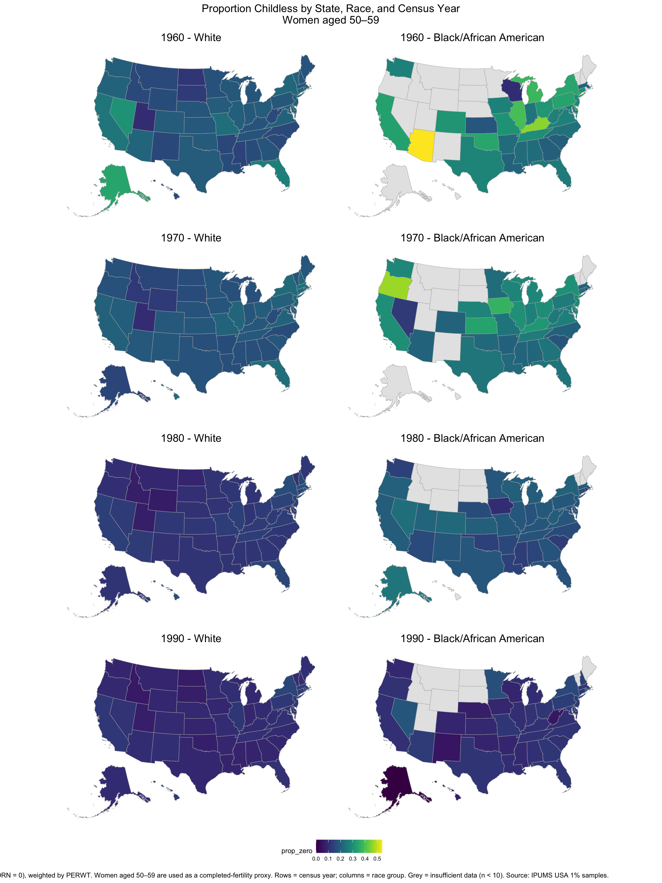

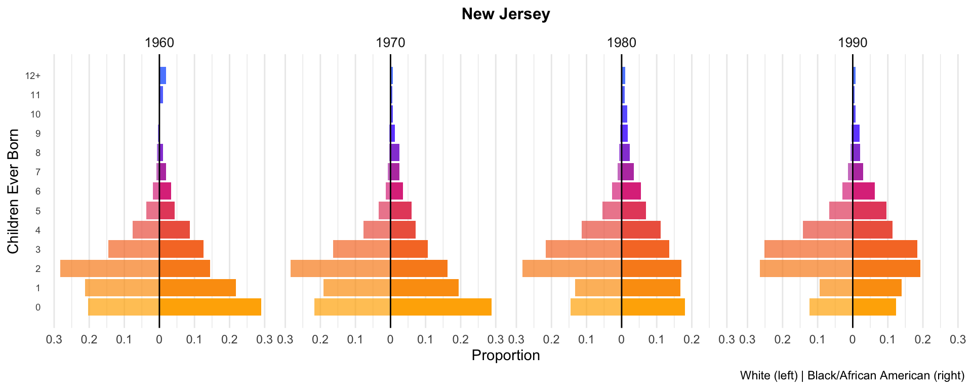
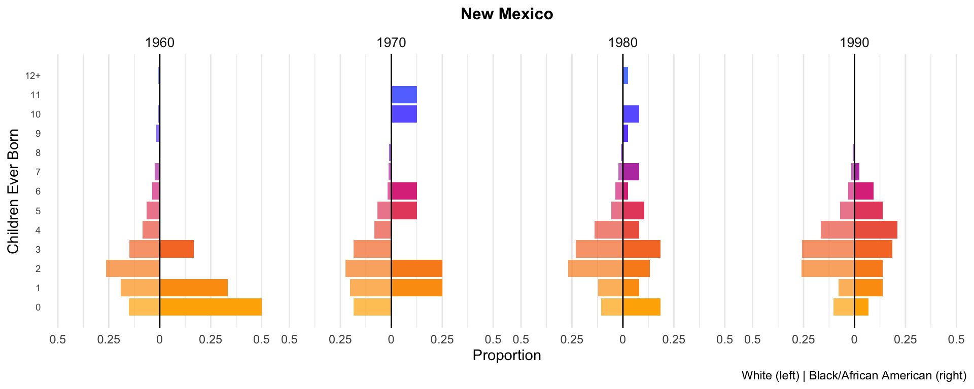
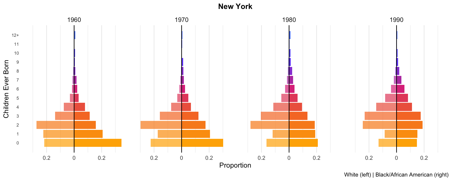
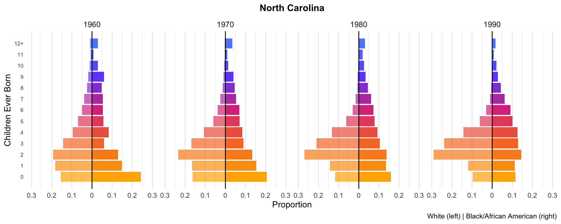
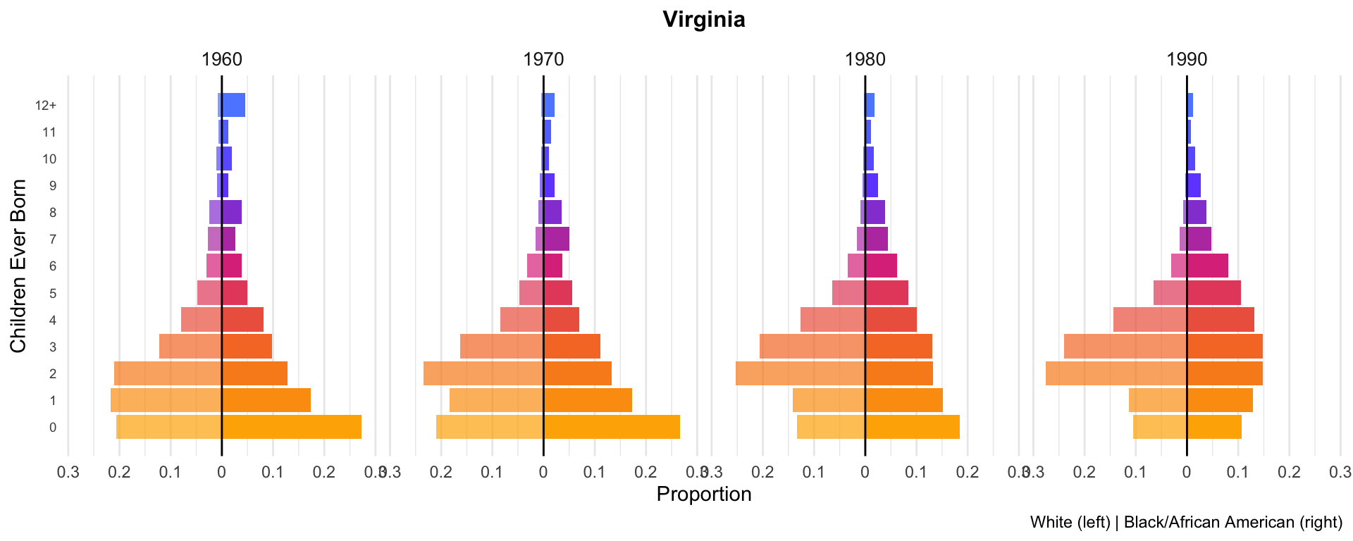
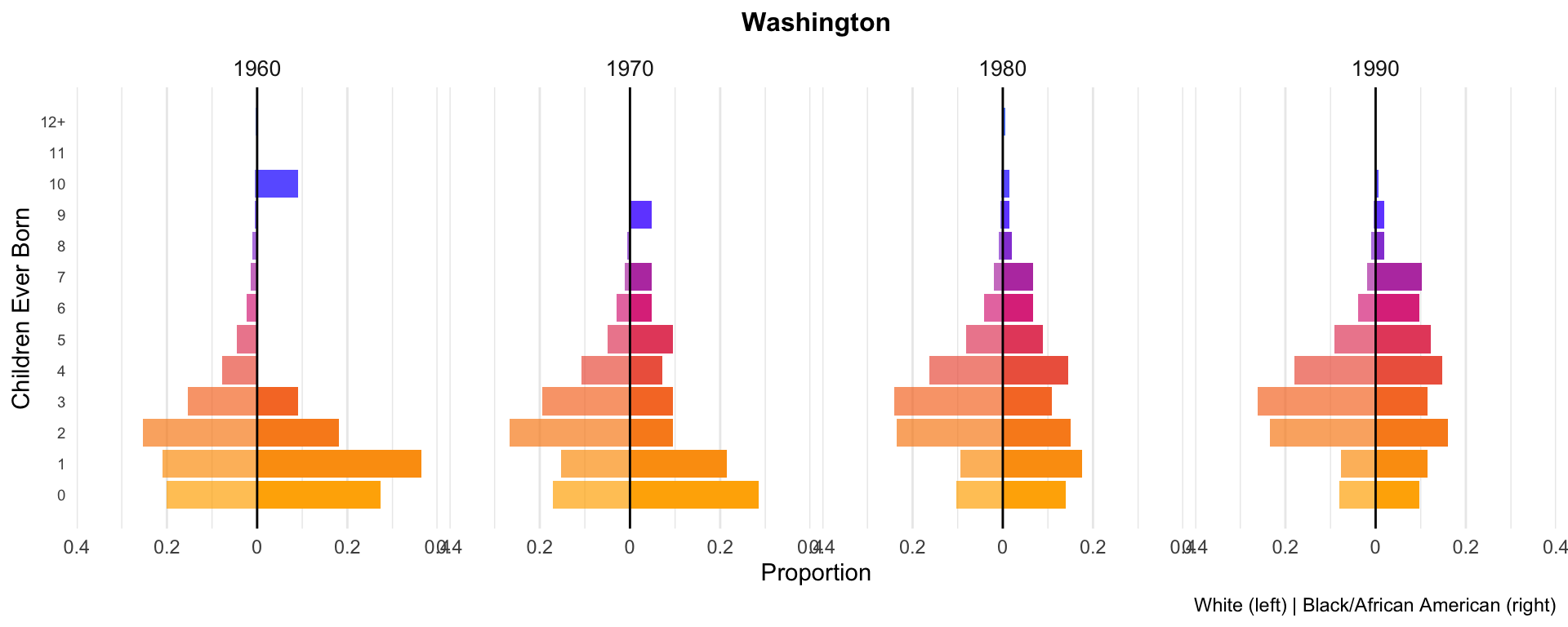
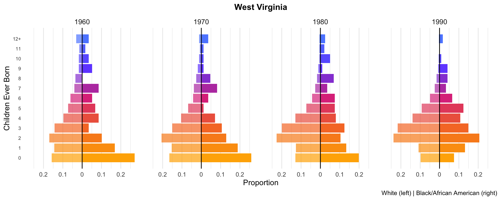
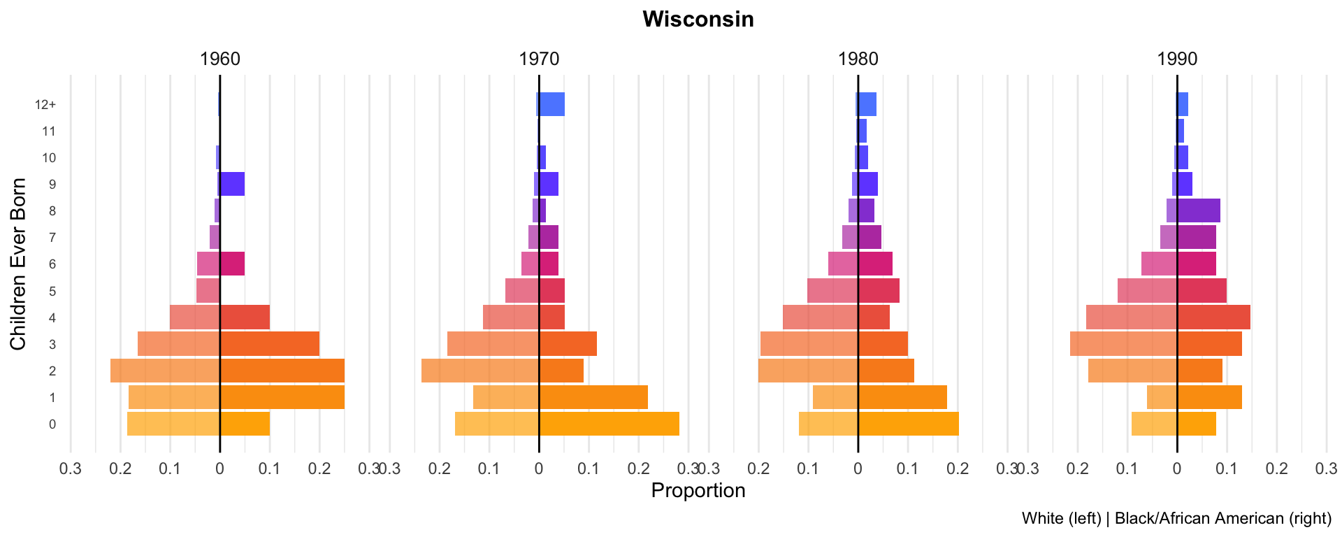
Past versions of map-zero-inflation-1.png

Version	Author	Date
71cf78a	Tina Lasisi	2026-04-14
bede61f	Tina Lasisi	2026-04-14

7. Per-state mirrored bar charts

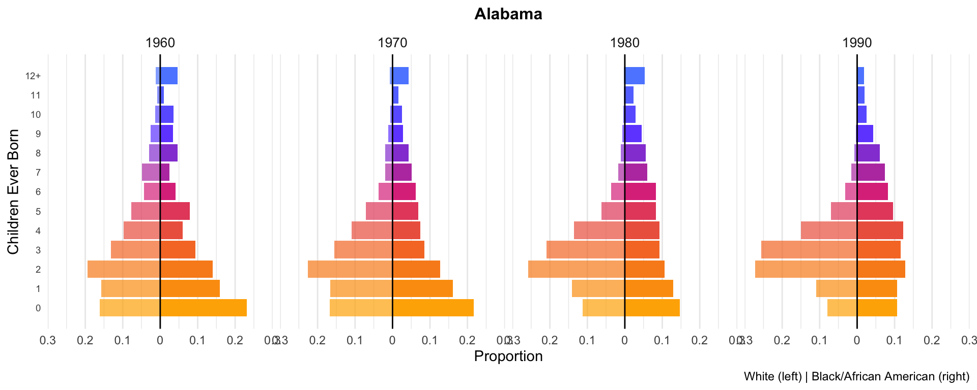
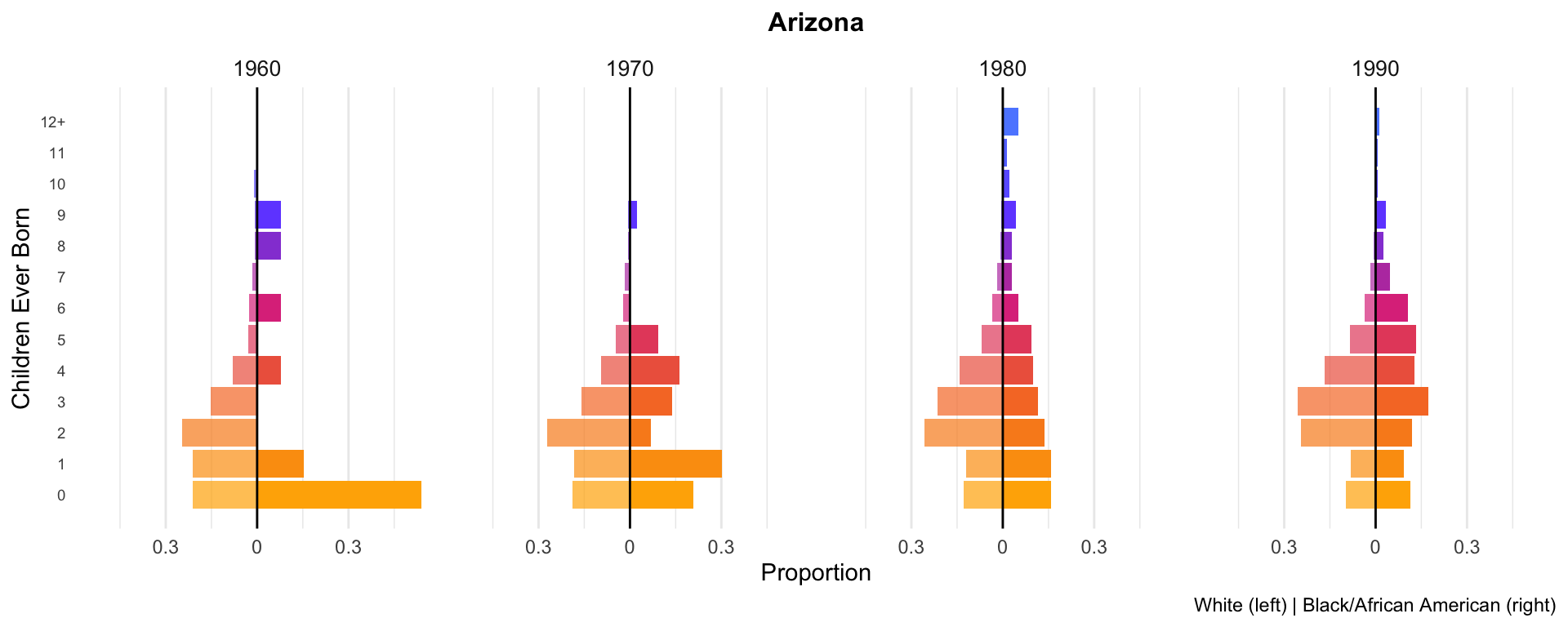
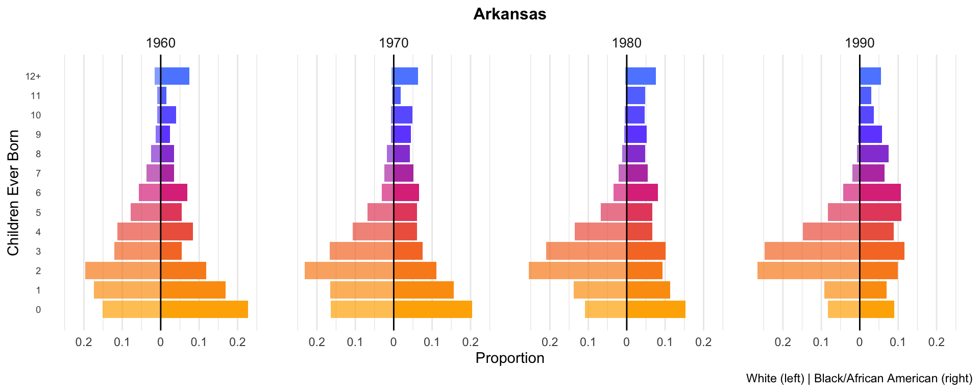
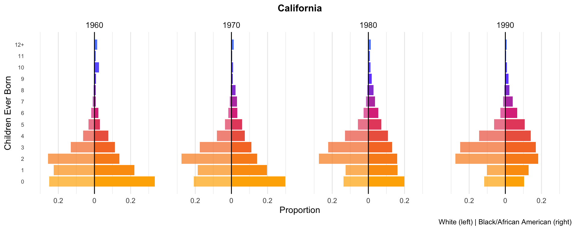
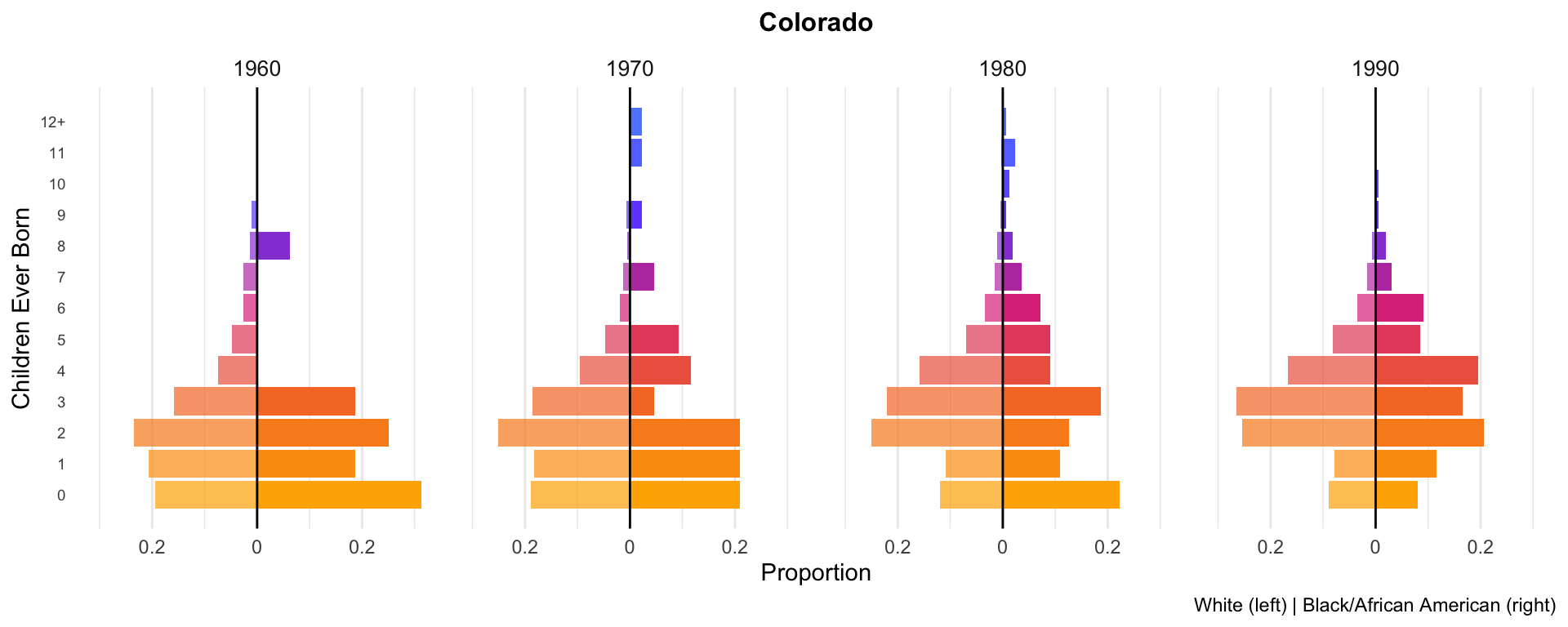
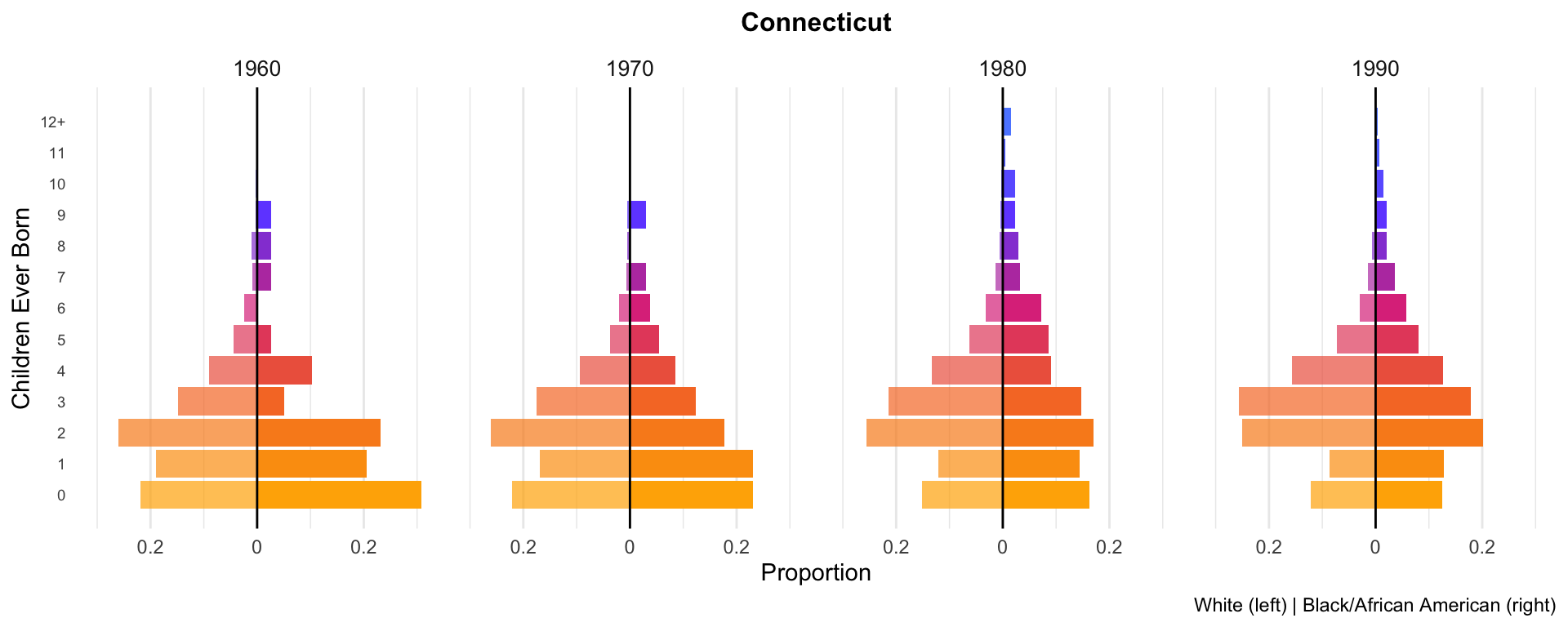
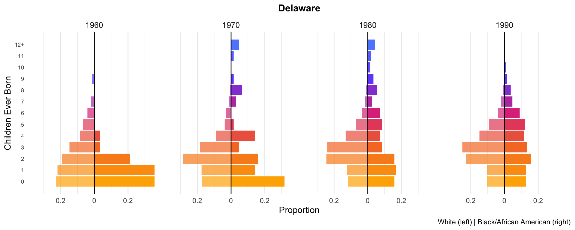
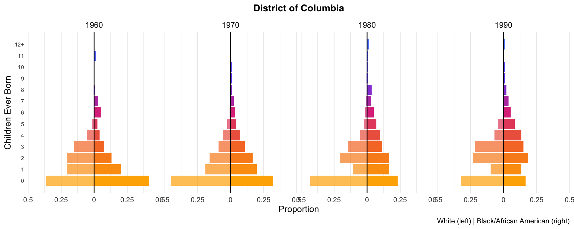
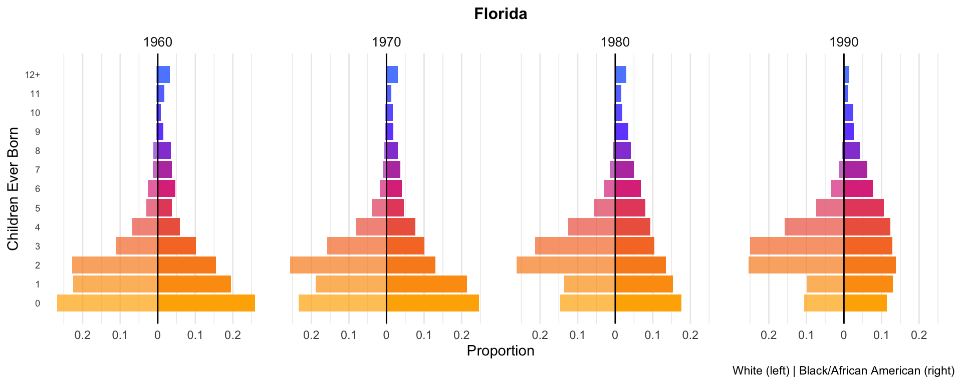
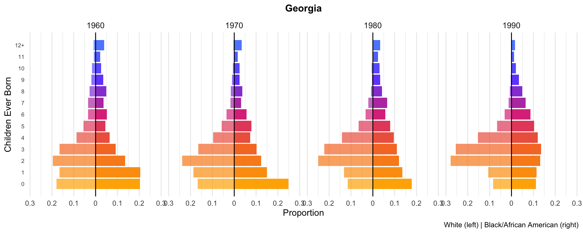
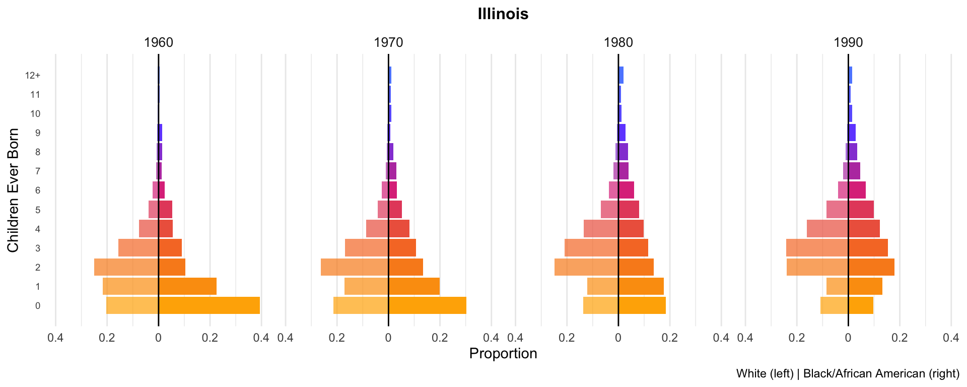
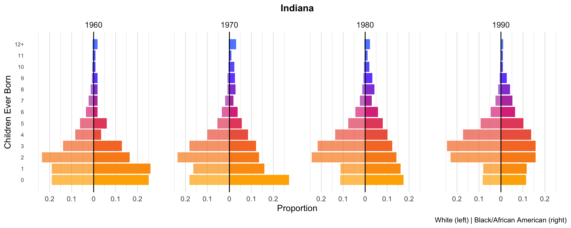
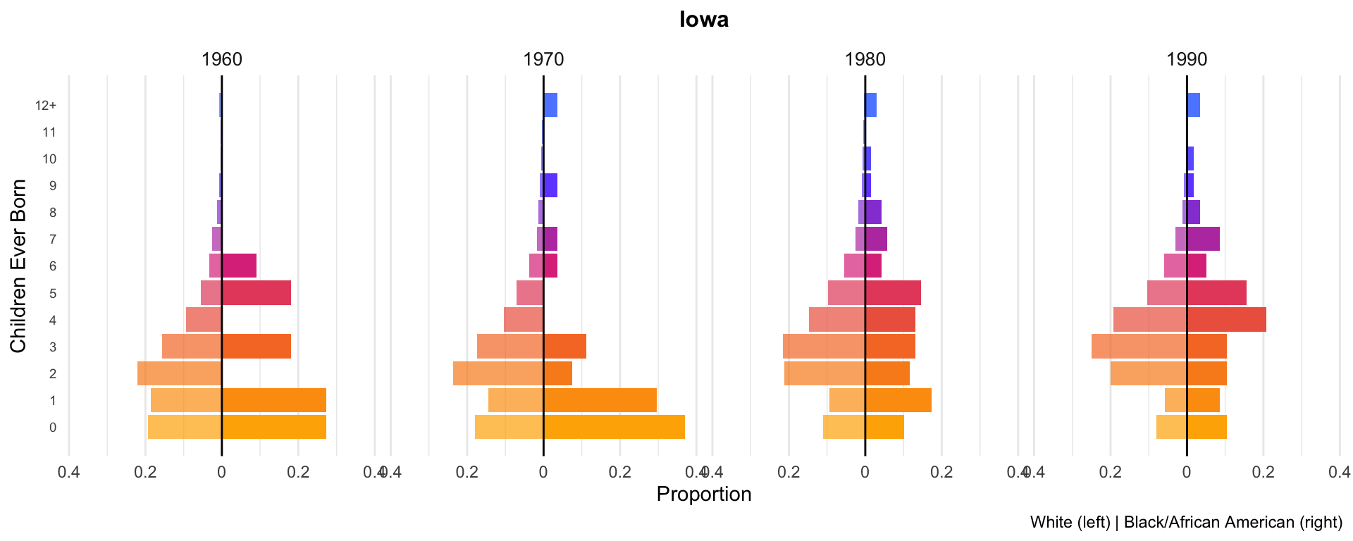
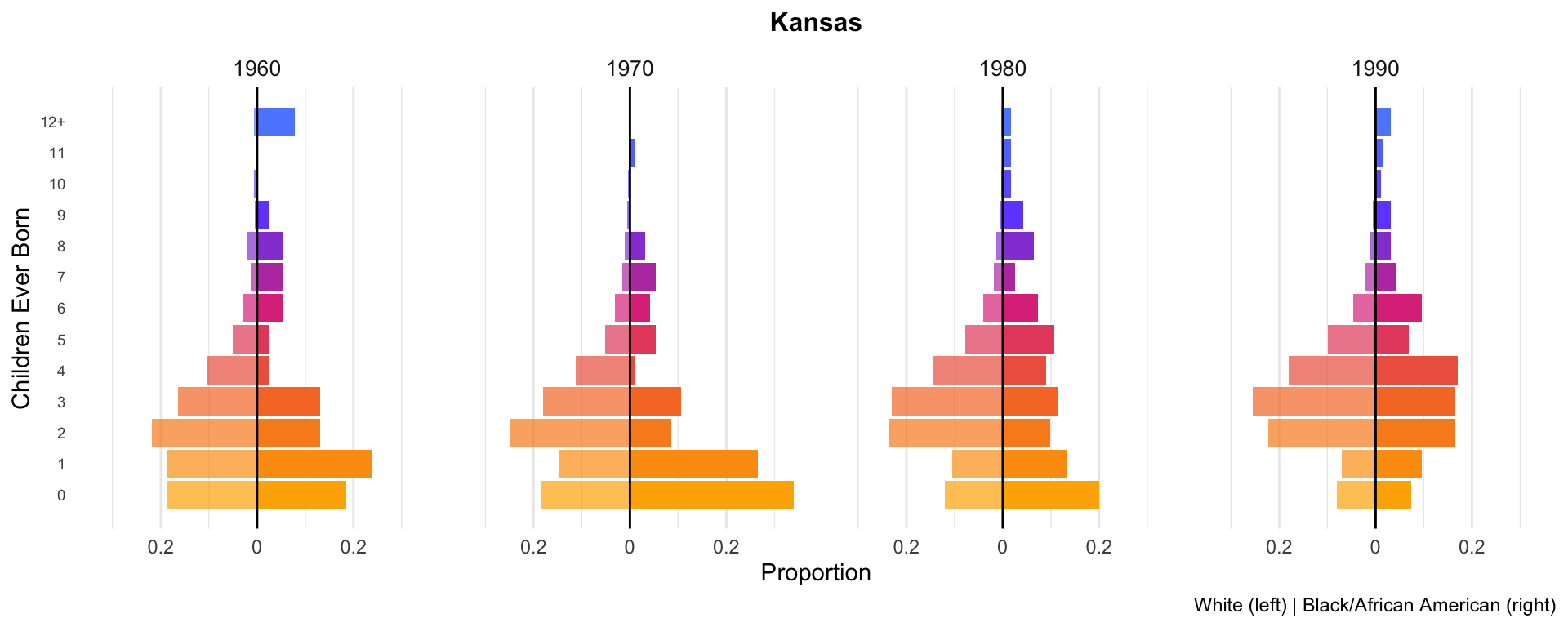
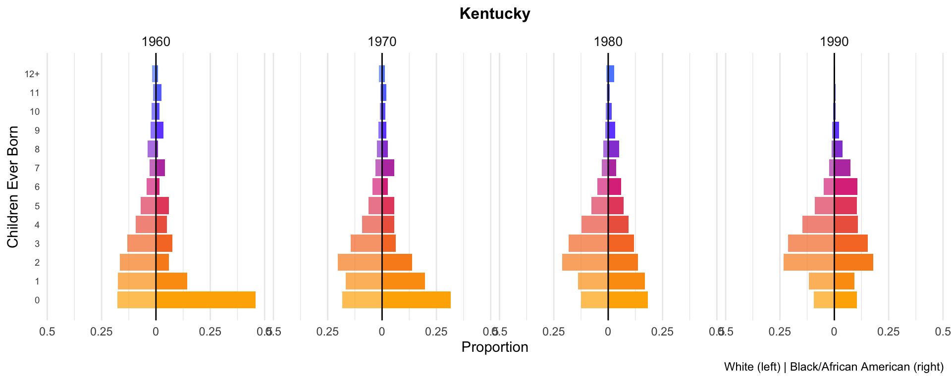
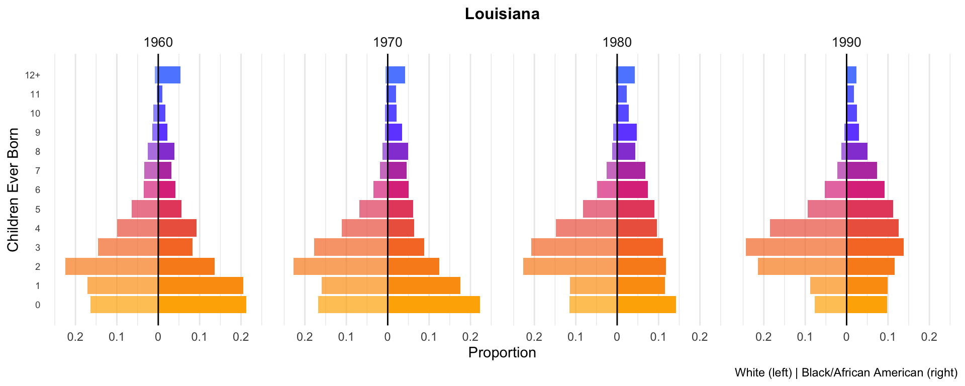
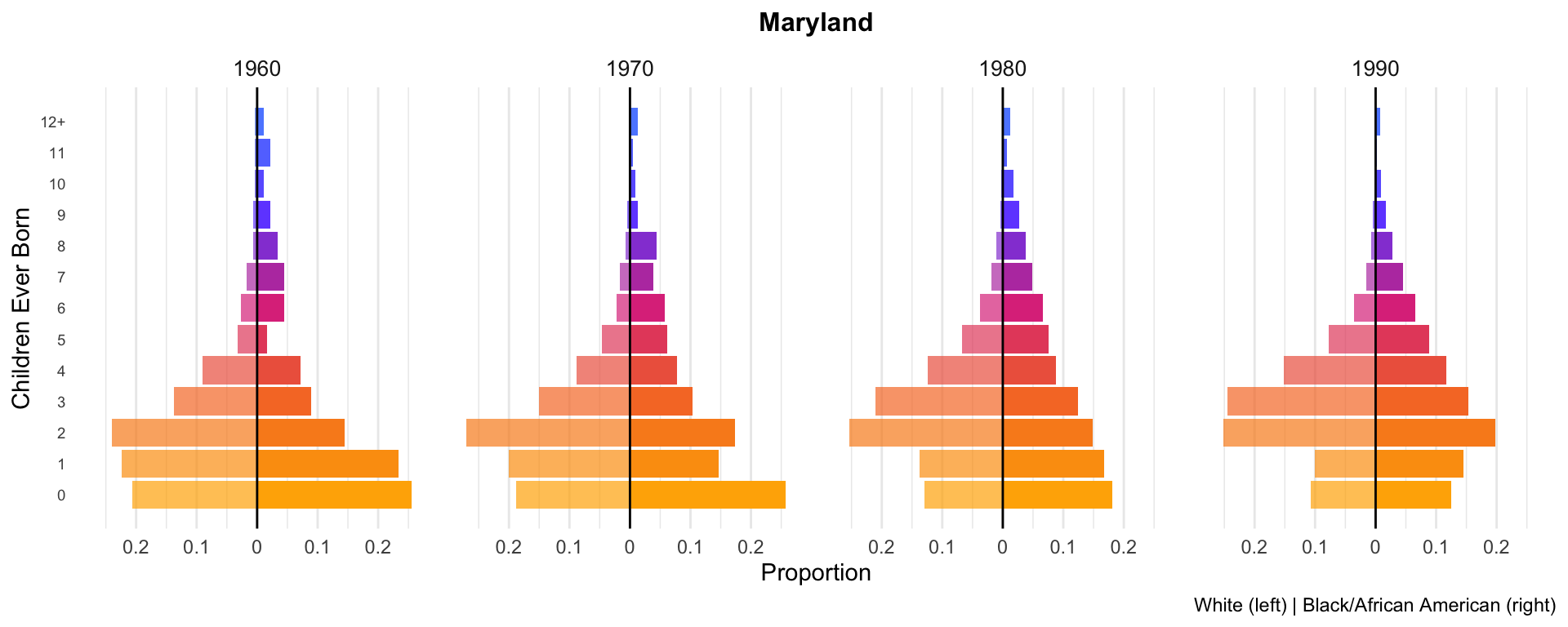
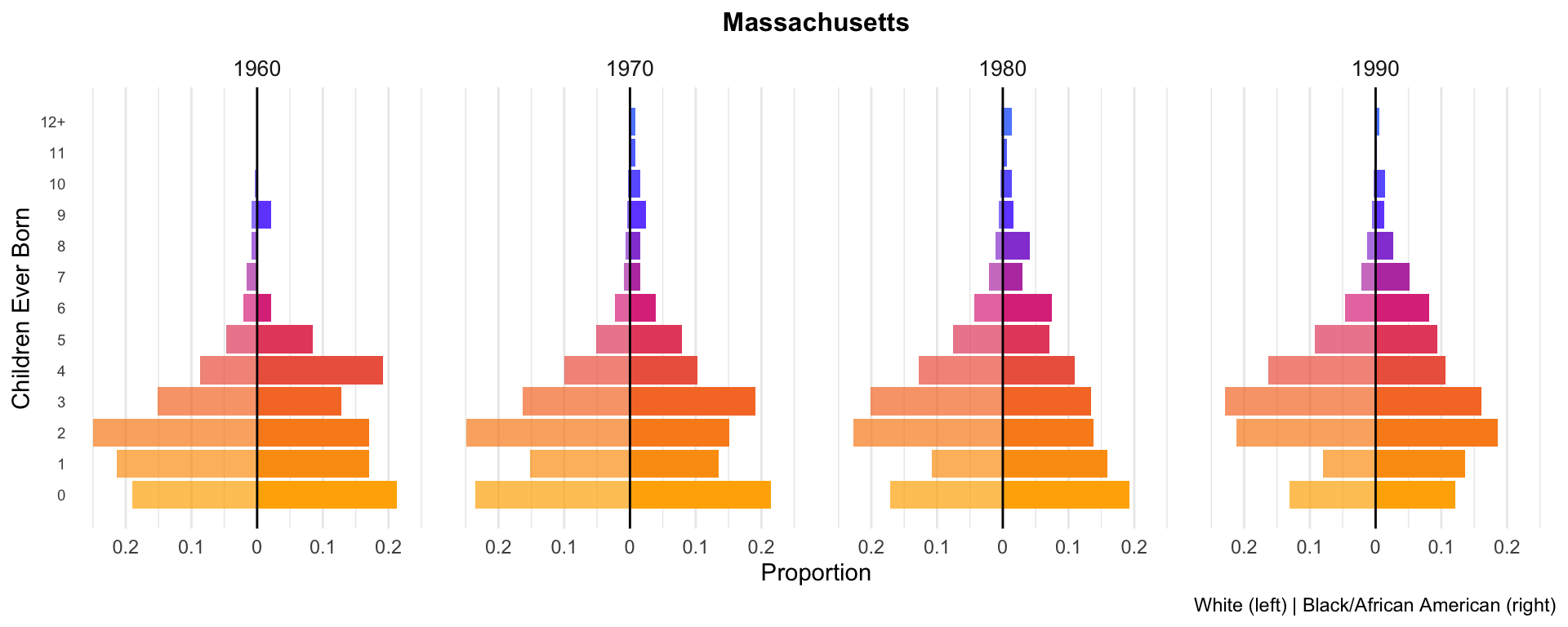
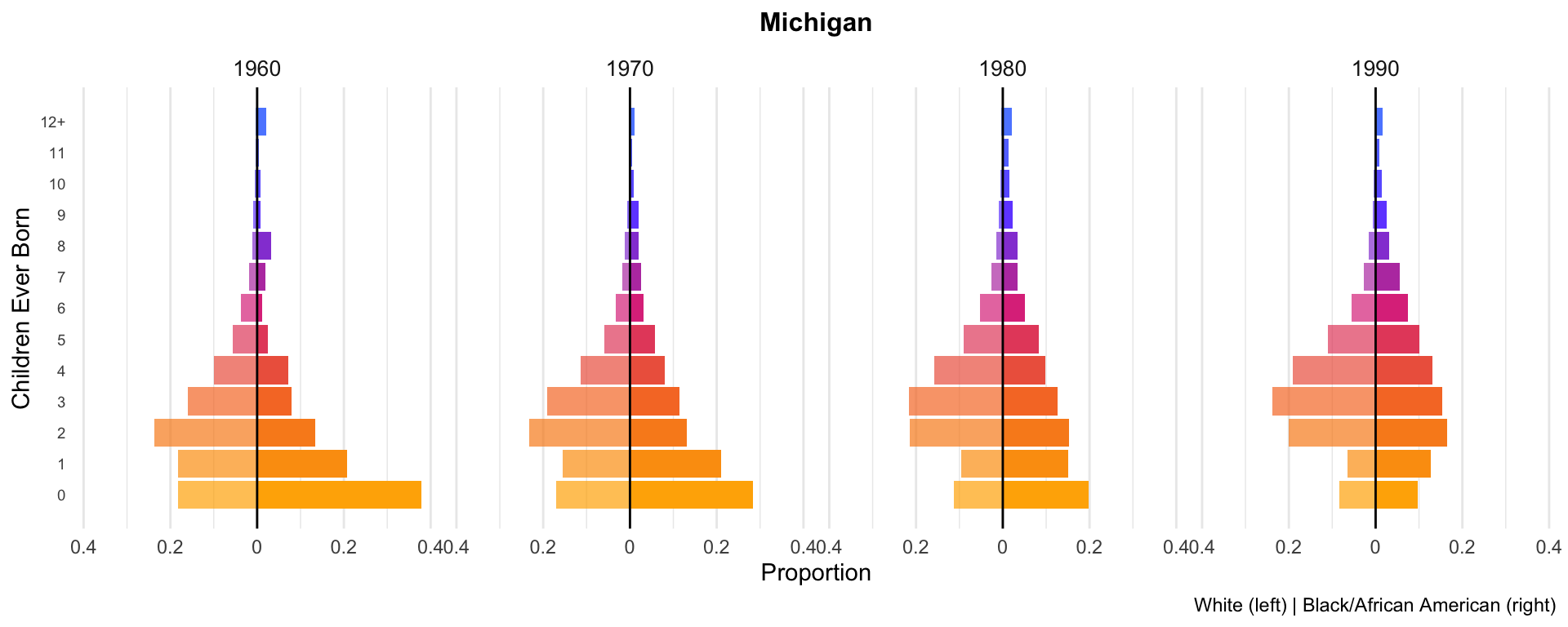
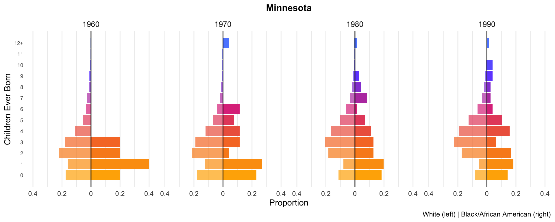
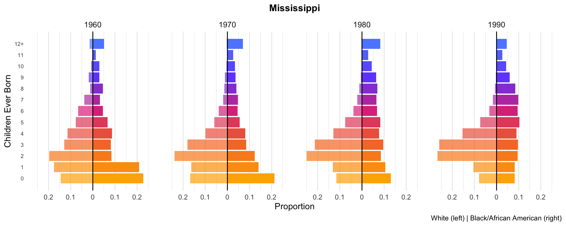
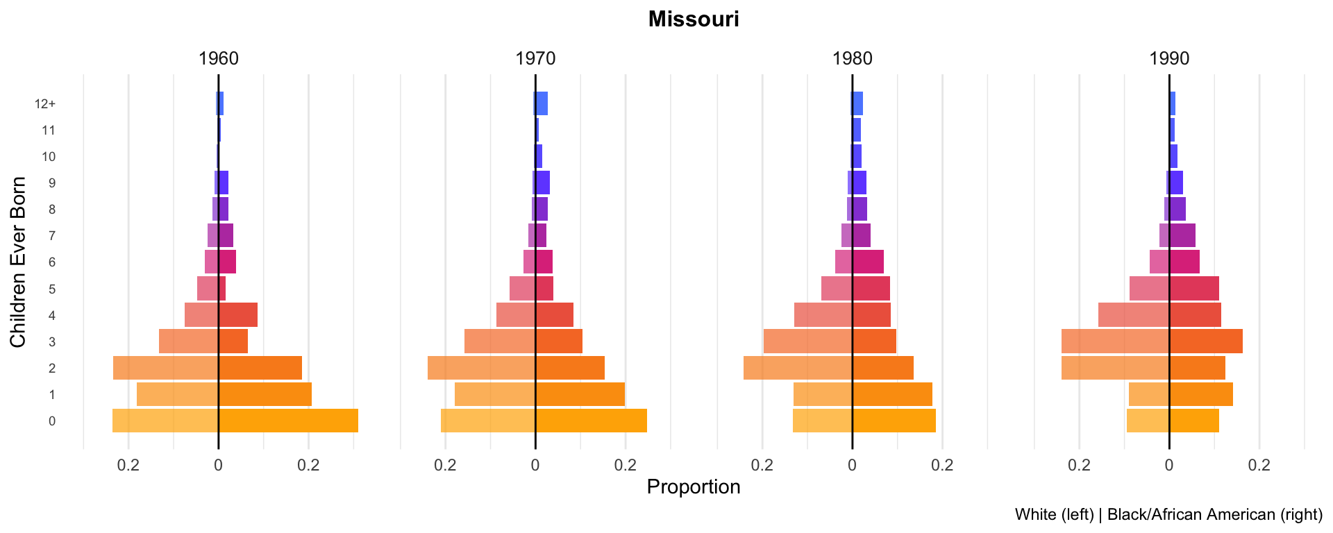
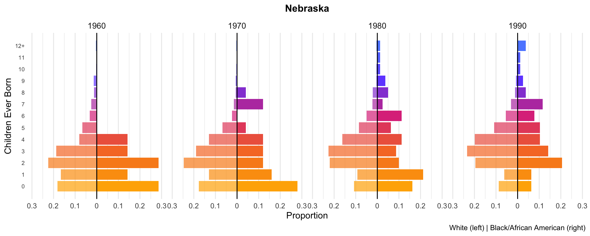
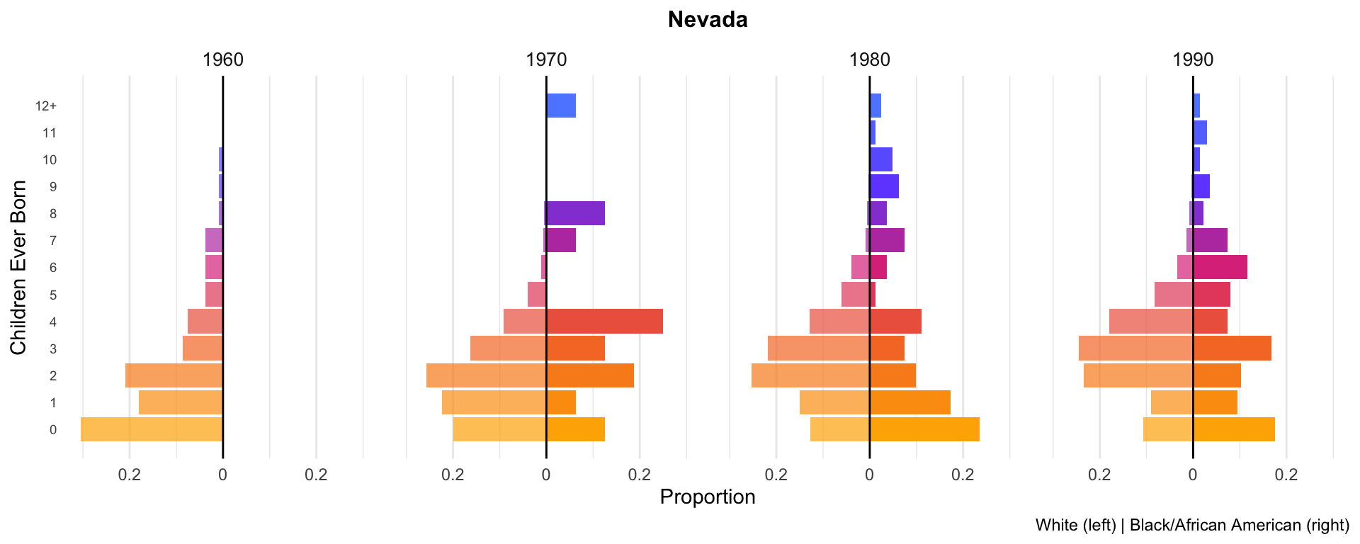
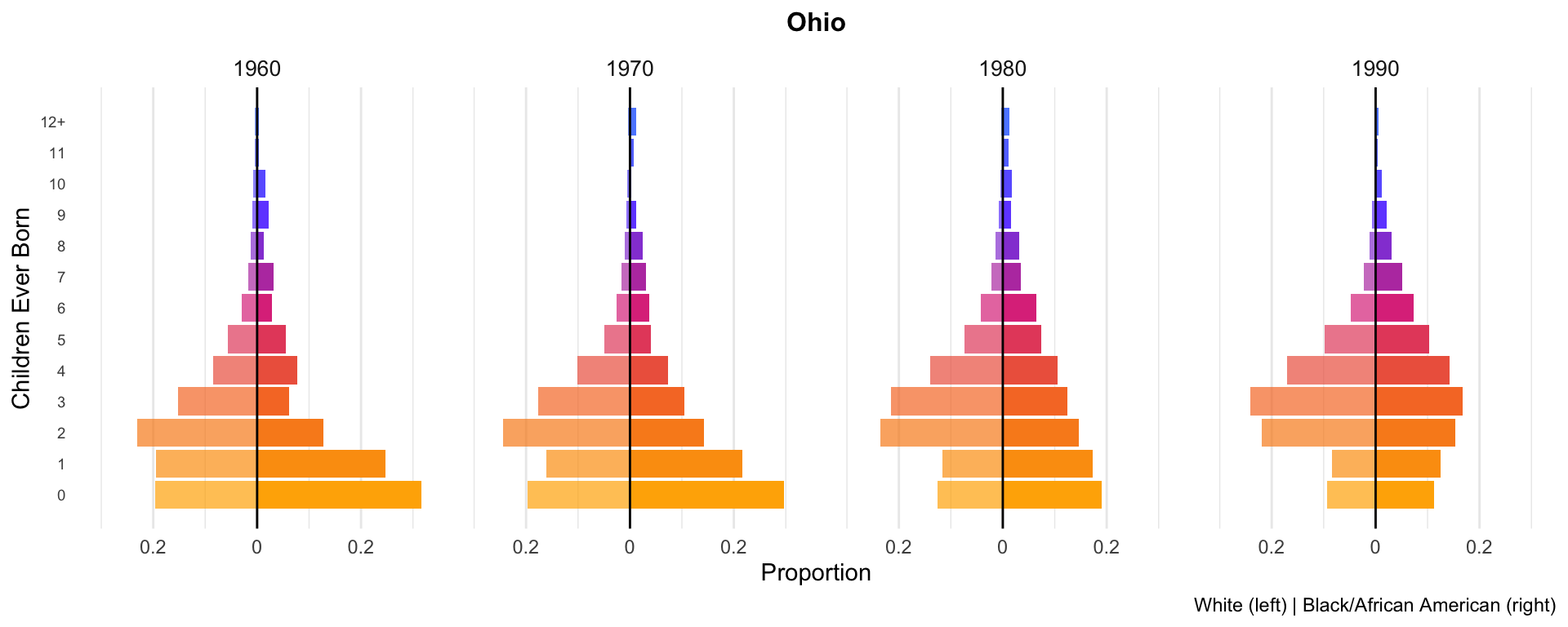
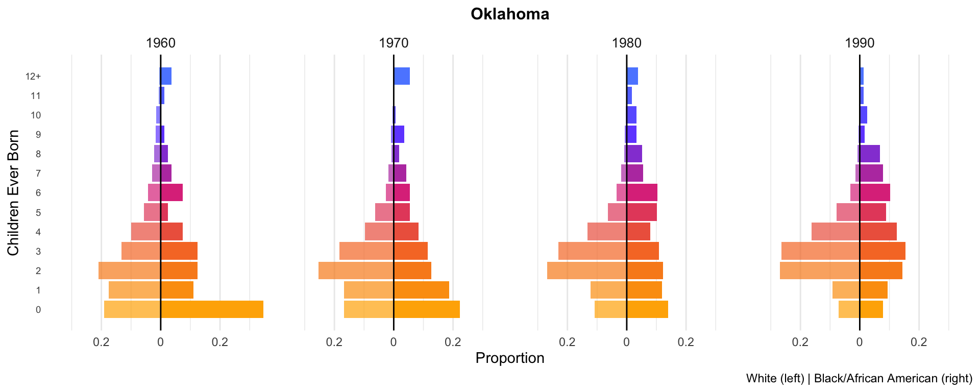
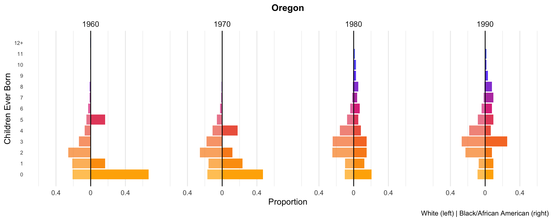
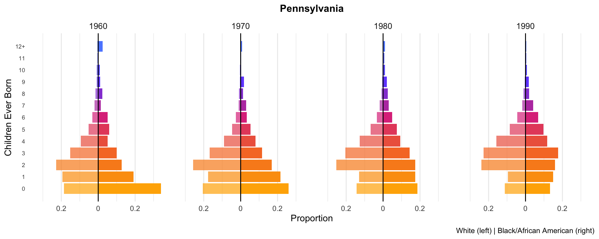
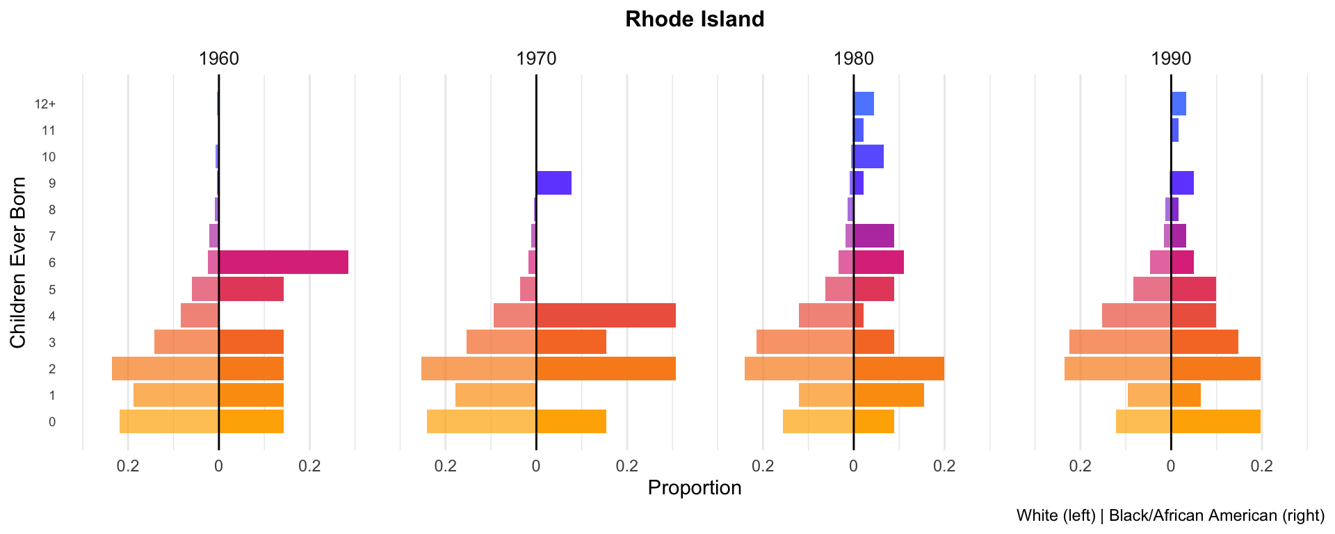
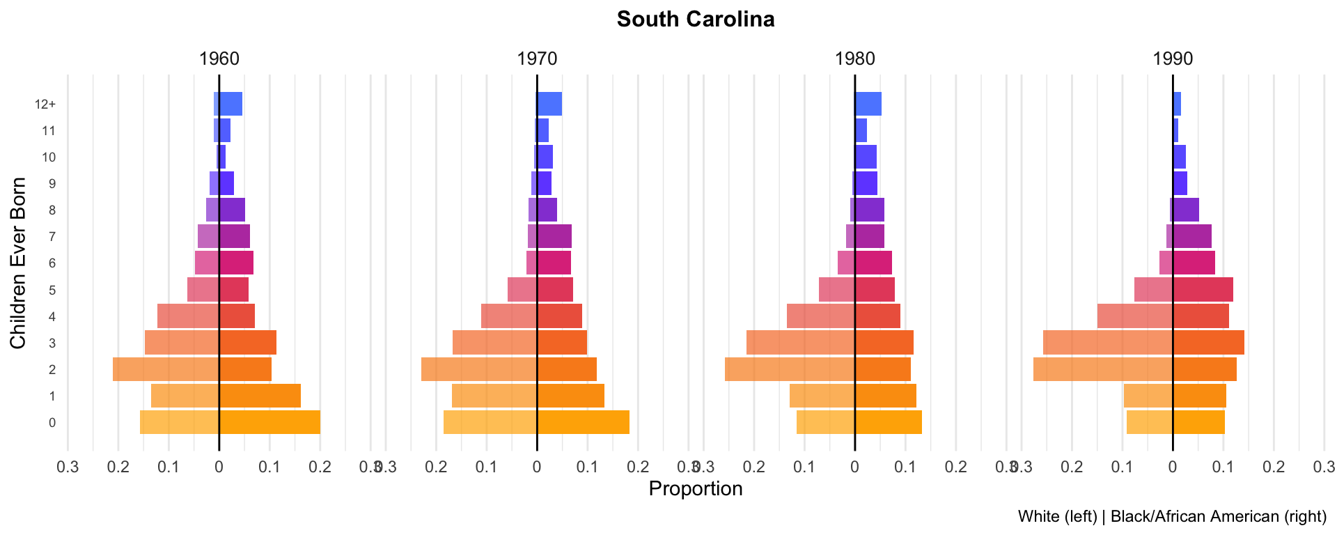
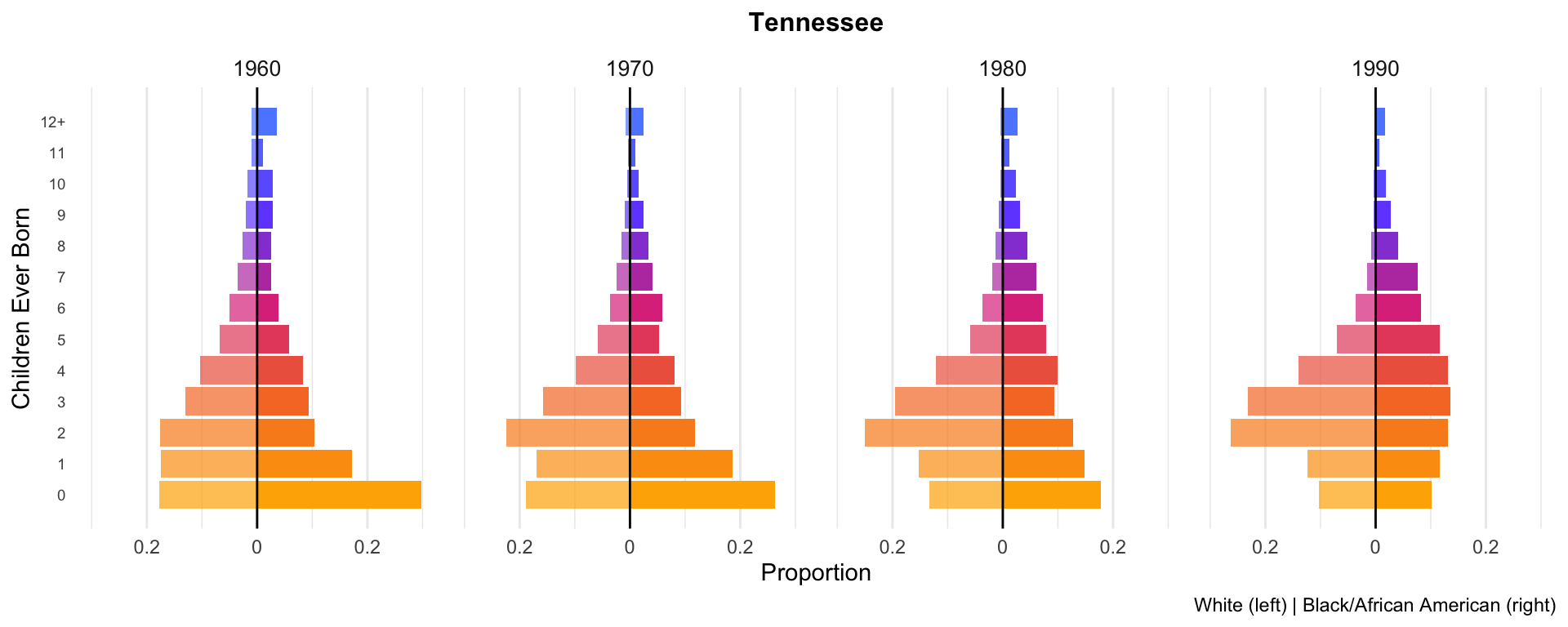
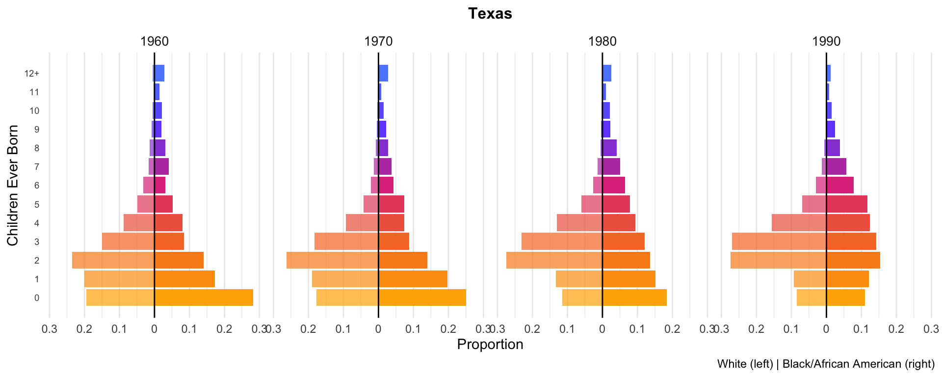
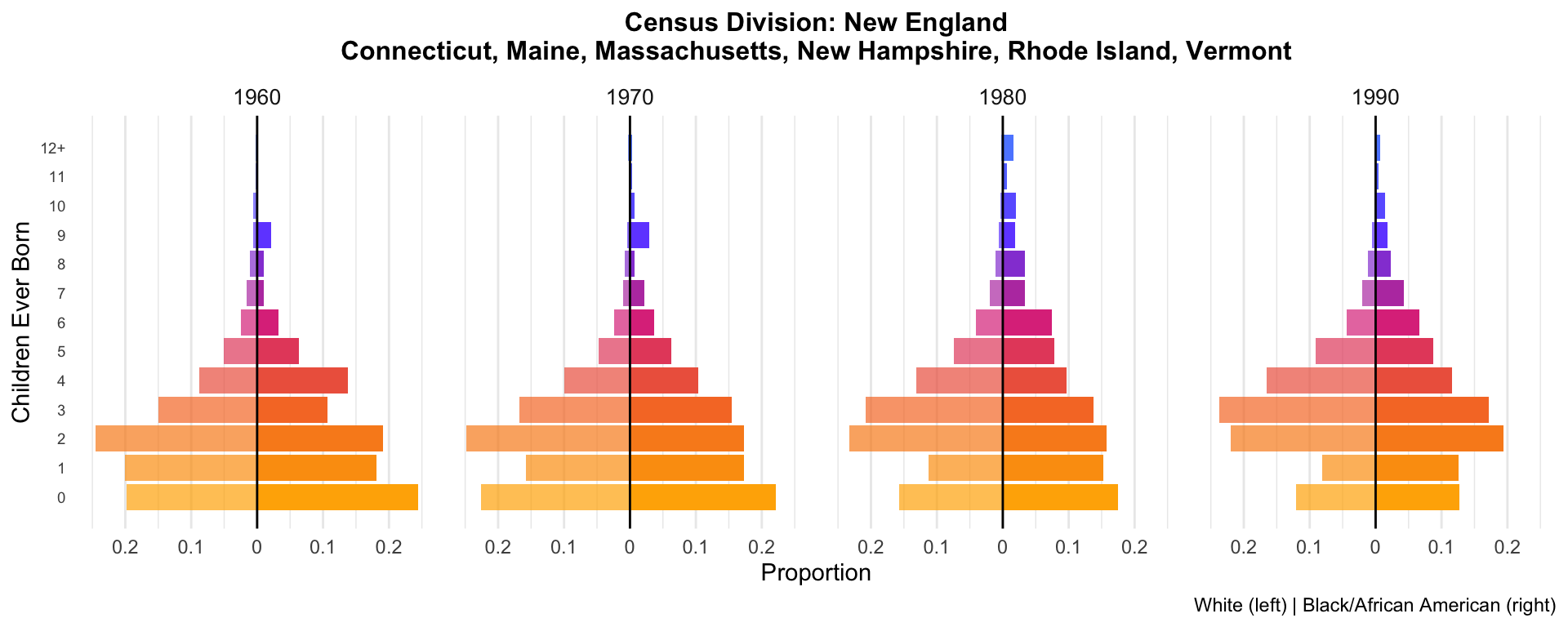
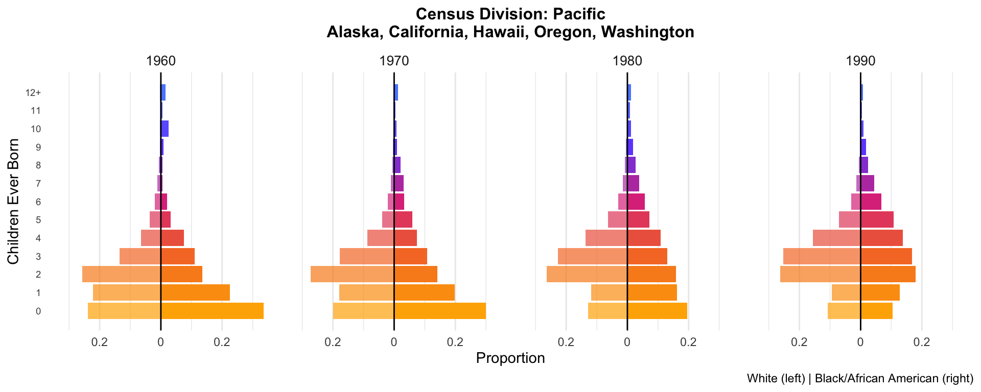
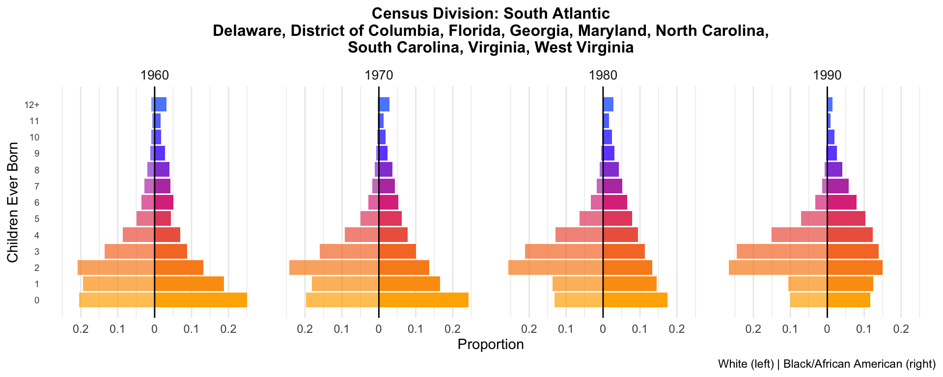
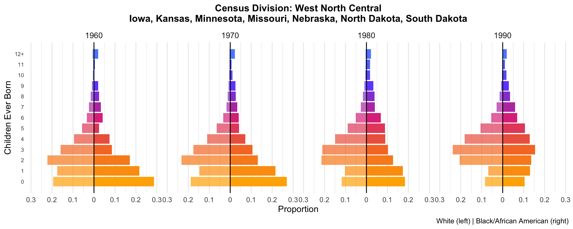
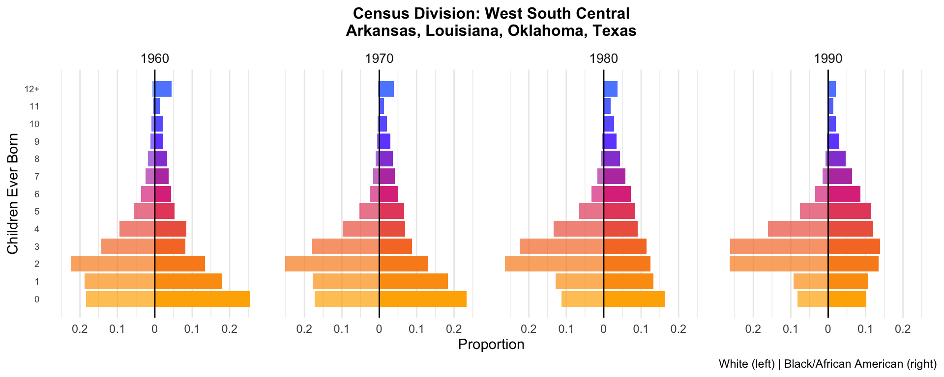
These detailed plots show the full distribution of children ever born for each state, using the same mirrored bar chart design as the national analysis: White proportions extend left, Black/African American proportions extend right.

Only states with at least 30 observations for both race groups across all included years are shown.

my_colors <- fertility_palette(13)

plot_state_fertility <- function(state_data, state_label) {
  # Compute proportions within each (YEAR, RACE) group
  df_props <- state_data %>%
    group_by(YEAR, RACE, chborn_capped) %>%
    summarise(count = n(), .groups = "drop") %>%
    group_by(YEAR, RACE) %>%
    mutate(proportion = count / sum(count)) %>%
    ungroup() %>%
    mutate(proportion = if_else(RACE == "White", -proportion, proportion))

  ggplot(df_props, aes(x = chborn_capped, y = proportion,
                       fill = as.factor(chborn_capped))) +
    geom_col(aes(alpha = RACE)) +
    geom_hline(yintercept = 0, color = "black", linewidth = 0.5) +
    facet_wrap(~ YEAR, nrow = 1) +
    coord_flip() +
    scale_y_continuous(
      labels = function(x) abs(x),
      limits = function(x) c(-max(abs(x)), max(abs(x)))
    ) +
    scale_x_continuous(breaks = 0:12, labels = c(0:11, "12+")) +
    scale_fill_manual(values = my_colors) +
    scale_alpha_manual(
      values = c("White" = 0.7, "Black/African American" = 1),
      guide = "none"
    ) +
    labs(
      title = state_label,
      x = "Children Ever Born",
      y = "Proportion",
      caption = "White (left) | Black/African American (right)"
    ) +
    theme_minimal() +
    theme(
      plot.title = element_text(size = 12, hjust = 0.5, face = "bold"),
      axis.text.y = element_text(size = 7),
      strip.text = element_text(size = 10),
      legend.position = "none",
      panel.grid.major.y = element_blank(),
      panel.grid.minor.y = element_blank()
    )
}

# States with >= 30 obs for both races in at least one year
eligible_states <- cell_sizes %>%
  filter(flag == "ok") %>%
  group_by(state_name) %>%
  filter(all(c("White", "Black/African American") %in% RACE)) %>%
  pull(state_name) %>%
  unique() %>%
  sort()

cat(length(eligible_states), "states with adequate data for both race groups:\n")

40 states with adequate data for both race groups:

cat(paste(eligible_states, collapse = ", "), "\n")

Alabama, Arizona, Arkansas, California, Colorado, Connecticut, Delaware, District of Columbia, Florida, Georgia, Illinois, Indiana, Iowa, Kansas, Kentucky, Louisiana, Maryland, Massachusetts, Michigan, Minnesota, Mississippi, Missouri, Nebraska, Nevada, New Jersey, New Mexico, New York, North Carolina, Ohio, Oklahoma, Oregon, Pennsylvania, Rhode Island, South Carolina, Tennessee, Texas, Virginia, Washington, West Virginia, Wisconsin 

for (st in eligible_states) {
  st_data <- data %>% filter(state_name == st)

  # Check both races are present
  if (n_distinct(st_data$RACE) < 2) next

  p <- plot_state_fertility(st_data, st)
  print(p)
  cat("\n\n")
}

Past versions of state-plots-1.png

Version	Author	Date
bede61f	Tina Lasisi	2026-04-14

Past versions of state-plots-2.png

Version	Author	Date
bede61f	Tina Lasisi	2026-04-14

Past versions of state-plots-3.png

Version	Author	Date
bede61f	Tina Lasisi	2026-04-14

Past versions of state-plots-4.png

Version	Author	Date
bede61f	Tina Lasisi	2026-04-14

Past versions of state-plots-5.png

Version	Author	Date
bede61f	Tina Lasisi	2026-04-14

Past versions of state-plots-6.png

Version	Author	Date
bede61f	Tina Lasisi	2026-04-14

Past versions of state-plots-7.png

Version	Author	Date
bede61f	Tina Lasisi	2026-04-14

Past versions of state-plots-8.png

Version	Author	Date
bede61f	Tina Lasisi	2026-04-14

Past versions of state-plots-9.png

Version	Author	Date
bede61f	Tina Lasisi	2026-04-14

Past versions of state-plots-10.png

Version	Author	Date
bede61f	Tina Lasisi	2026-04-14

Past versions of state-plots-11.png

Version	Author	Date
bede61f	Tina Lasisi	2026-04-14

Past versions of state-plots-12.png

Version	Author	Date
bede61f	Tina Lasisi	2026-04-14

Past versions of state-plots-13.png

Version	Author	Date
bede61f	Tina Lasisi	2026-04-14

Past versions of state-plots-14.png

Version	Author	Date
bede61f	Tina Lasisi	2026-04-14

Past versions of state-plots-15.png

Version	Author	Date
bede61f	Tina Lasisi	2026-04-14

Past versions of state-plots-16.png

Version	Author	Date
bede61f	Tina Lasisi	2026-04-14

Past versions of state-plots-17.png

Version	Author	Date
bede61f	Tina Lasisi	2026-04-14

Past versions of state-plots-18.png

Version	Author	Date
bede61f	Tina Lasisi	2026-04-14

Past versions of state-plots-19.png

Version	Author	Date
bede61f	Tina Lasisi	2026-04-14

Past versions of state-plots-20.png

Version	Author	Date
bede61f	Tina Lasisi	2026-04-14

Past versions of state-plots-21.png

Version	Author	Date
bede61f	Tina Lasisi	2026-04-14

Past versions of state-plots-22.png

Version	Author	Date
bede61f	Tina Lasisi	2026-04-14

Past versions of state-plots-23.png

Version	Author	Date
bede61f	Tina Lasisi	2026-04-14

Past versions of state-plots-24.png

Version	Author	Date
bede61f	Tina Lasisi	2026-04-14

Past versions of state-plots-25.png

Version	Author	Date
bede61f	Tina Lasisi	2026-04-14

Past versions of state-plots-26.png

Version	Author	Date
bede61f	Tina Lasisi	2026-04-14

Past versions of state-plots-27.png

Version	Author	Date
bede61f	Tina Lasisi	2026-04-14

Past versions of state-plots-28.png

Version	Author	Date
bede61f	Tina Lasisi	2026-04-14

Past versions of state-plots-29.png

Version	Author	Date
bede61f	Tina Lasisi	2026-04-14

Past versions of state-plots-30.png

Version	Author	Date
bede61f	Tina Lasisi	2026-04-14

Past versions of state-plots-31.png

Version	Author	Date
bede61f	Tina Lasisi	2026-04-14

Past versions of state-plots-32.png

Version	Author	Date
bede61f	Tina Lasisi	2026-04-14

Past versions of state-plots-33.png

Version	Author	Date
bede61f	Tina Lasisi	2026-04-14

Past versions of state-plots-34.png

Version	Author	Date
bede61f	Tina Lasisi	2026-04-14

Past versions of state-plots-35.png

Version	Author	Date
bede61f	Tina Lasisi	2026-04-14

Past versions of state-plots-36.png

Version	Author	Date
bede61f	Tina Lasisi	2026-04-14

Past versions of state-plots-37.png

Version	Author	Date
bede61f	Tina Lasisi	2026-04-14

Past versions of state-plots-38.png

Version	Author	Date
bede61f	Tina Lasisi	2026-04-14

Past versions of state-plots-39.png

Version	Author	Date
bede61f	Tina Lasisi	2026-04-14

Past versions of state-plots-40.png

Version	Author	Date
bede61f	Tina Lasisi	2026-04-14

8. Regional aggregation: Census divisions

For states where the Black/African American sample is too small, we aggregate to Census divisions and produce division-level plots.

Census divisions and their member states:

• New England: Connecticut, Maine, Massachusetts, New Hampshire, Rhode Island, Vermont
• Middle Atlantic: New Jersey, New York, Pennsylvania
• East North Central: Illinois, Indiana, Michigan, Ohio, Wisconsin
• West North Central: Iowa, Kansas, Minnesota, Missouri, Nebraska, North Dakota, South Dakota
• South Atlantic: Delaware, District of Columbia, Florida, Georgia, Maryland, North Carolina, South Carolina, Virginia, West Virginia
• East South Central: Alabama, Kentucky, Mississippi, Tennessee
• West South Central: Arkansas, Louisiana, Oklahoma, Texas
• Mountain: Arizona, Colorado, Idaho, Montana, Nevada, New Mexico, Utah, Wyoming
• Pacific: Alaska, California, Hawaii, Oregon, Washington

data_with_division <- data %>%
  mutate(division = state_to_division(state_name))

# Division-level cell sizes
div_cells <- data_with_division %>%
  count(division, RACE, YEAR, name = "n_obs") %>%
  filter(!is.na(division))

# All divisions should have adequate sample sizes
div_eligible <- div_cells %>%
  filter(n_obs >= 30) %>%
  group_by(division) %>%
  filter(all(c("White", "Black/African American") %in% RACE)) %>%
  pull(division) %>%
  unique() %>%
  sort()

cat(length(div_eligible), "Census divisions with adequate data:\n")

9 Census divisions with adequate data:

cat(paste(div_eligible, collapse = ", "), "\n")

East North Central, East South Central, Middle Atlantic, Mountain, New England, Pacific, South Atlantic, West North Central, West South Central 

for (div in div_eligible) {
  div_data <- data_with_division %>%
    filter(division == div) %>%
    mutate(chborn_capped = pmin(chborn_num, 12))

  if (n_distinct(div_data$RACE) < 2) next

  states_in_div <- sort(unique(div_data$state_name))
  plot_title <- paste0("Census Division: ", div, "\n",
                       str_wrap(paste(states_in_div, collapse = ", "), width = 80))
  p <- plot_state_fertility(div_data, plot_title)
  print(p)
  cat("\n\n")
}

Past versions of division-plots-1.png

Version	Author	Date
9d44b29	Tina Lasisi	2026-04-14
bede61f	Tina Lasisi	2026-04-14

Past versions of division-plots-2.png

Version	Author	Date
9d44b29	Tina Lasisi	2026-04-14
bede61f	Tina Lasisi	2026-04-14

Past versions of division-plots-3.png

Version	Author	Date
9d44b29	Tina Lasisi	2026-04-14
bede61f	Tina Lasisi	2026-04-14

Past versions of division-plots-4.png

Version	Author	Date
9d44b29	Tina Lasisi	2026-04-14
bede61f	Tina Lasisi	2026-04-14

Past versions of division-plots-5.png

Version	Author	Date
9d44b29	Tina Lasisi	2026-04-14
bede61f	Tina Lasisi	2026-04-14

Past versions of division-plots-6.png

Version	Author	Date
9d44b29	Tina Lasisi	2026-04-14
bede61f	Tina Lasisi	2026-04-14

Past versions of division-plots-7.png

Version	Author	Date
9d44b29	Tina Lasisi	2026-04-14
bede61f	Tina Lasisi	2026-04-14

Past versions of division-plots-8.png

Version	Author	Date
9d44b29	Tina Lasisi	2026-04-14
bede61f	Tina Lasisi	2026-04-14

Past versions of division-plots-9.png

Version	Author	Date
9d44b29	Tina Lasisi	2026-04-14
bede61f	Tina Lasisi	2026-04-14

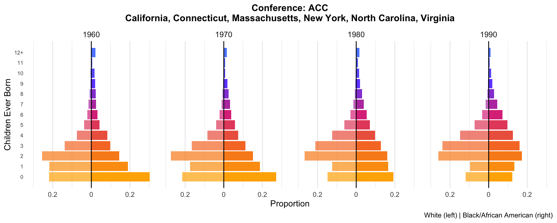
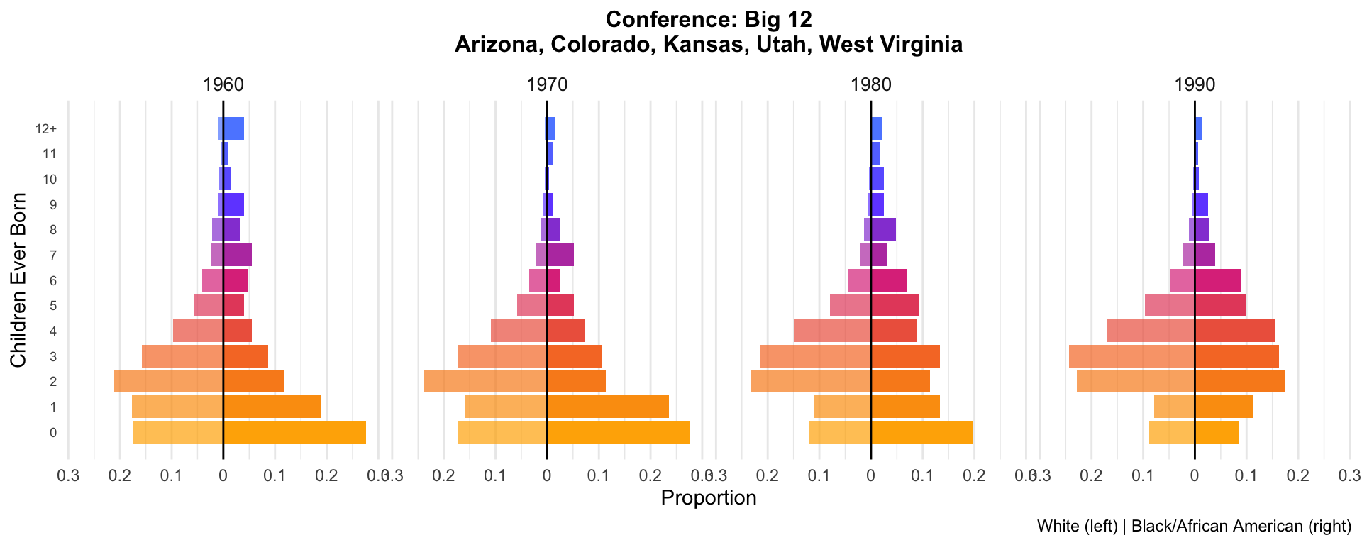
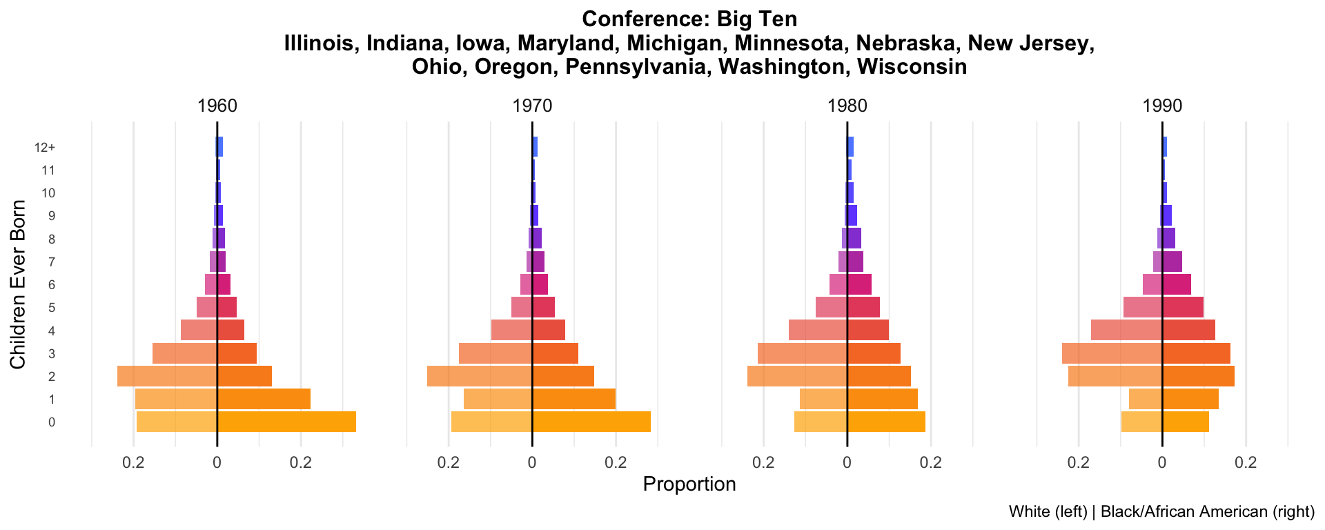
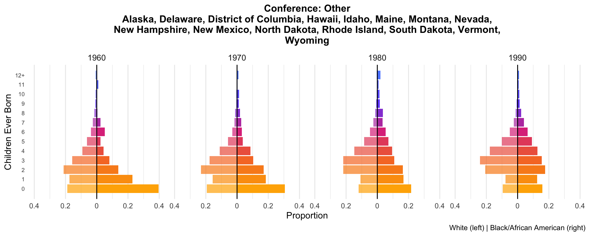
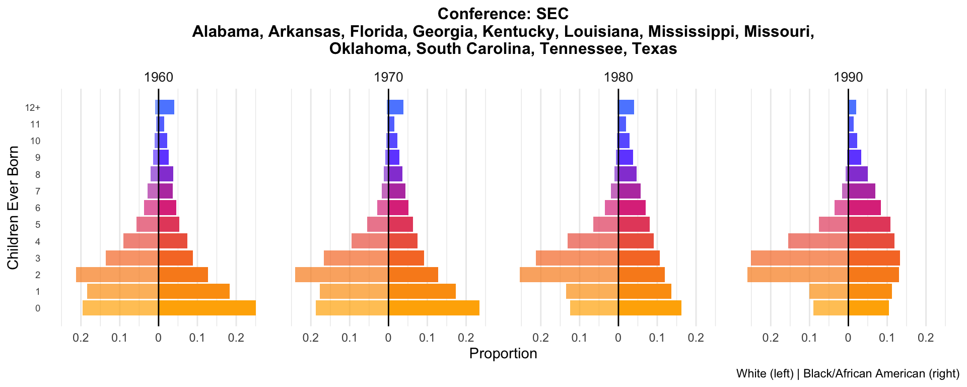
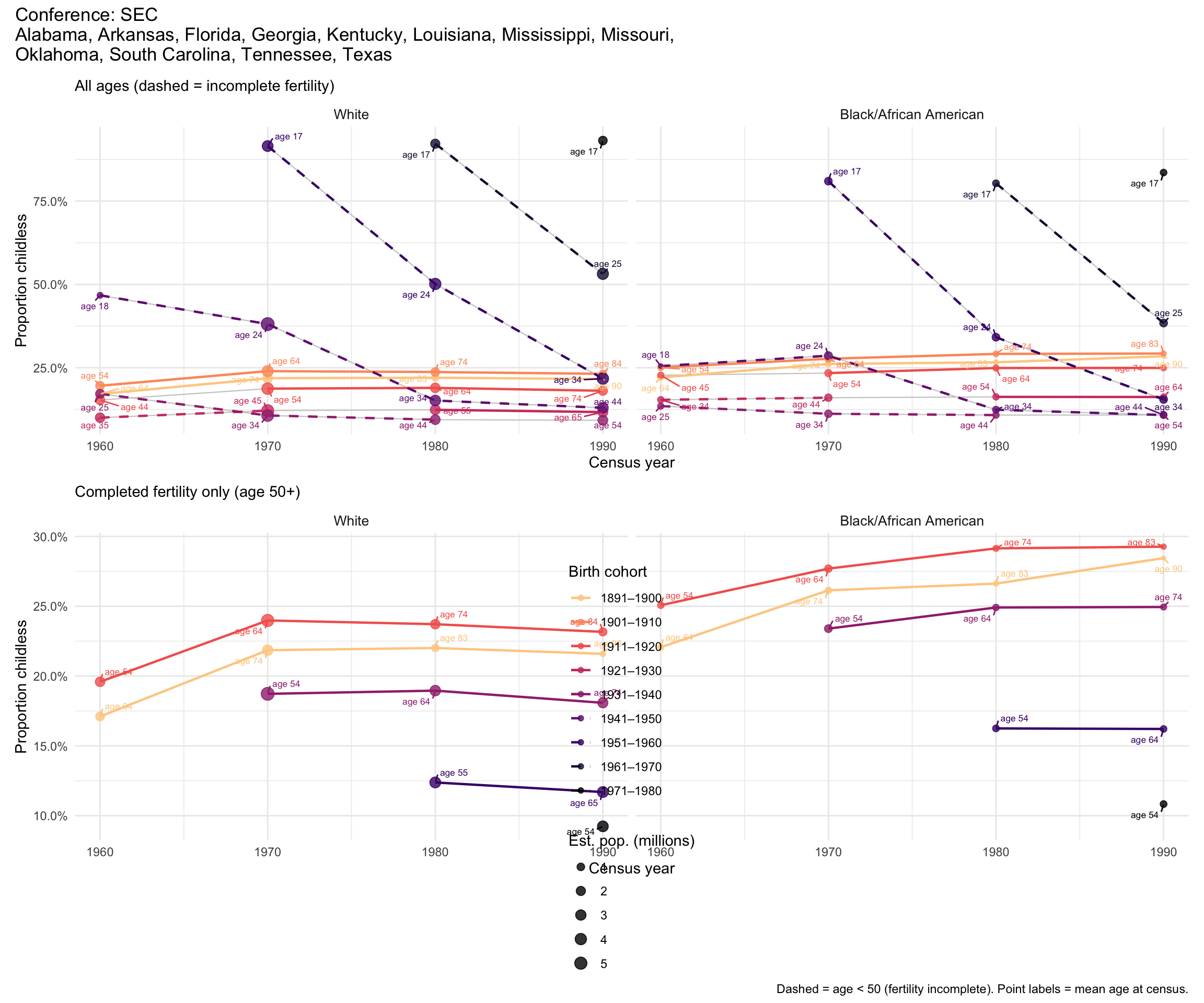
8b. Regional aggregation: College sports conferences

An alternative regional grouping based on major college athletic conferences, which reflect distinct cultural and geographic regions.

Conference membership (flagship/dominant program per state, post-2024 realignment):

• SEC: Alabama, Arkansas, Florida, Georgia, Kentucky, Louisiana, Mississippi, Missouri, Oklahoma, South Carolina, Tennessee, Texas
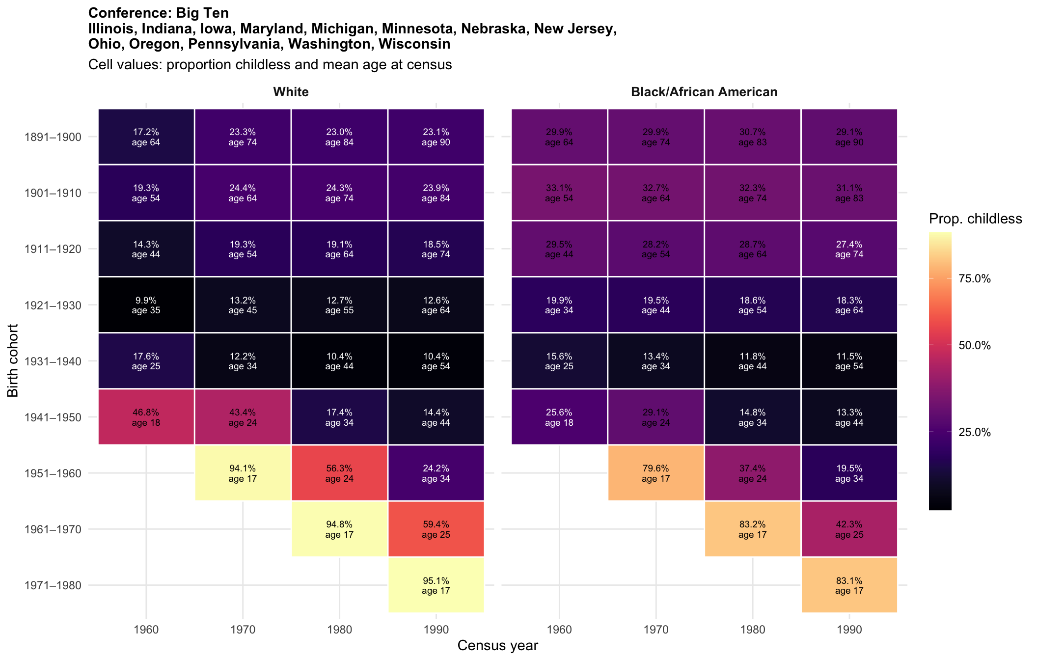
• Big Ten: Illinois, Indiana, Iowa, Maryland, Michigan, Minnesota, Nebraska, New Jersey, Ohio, Oregon, Pennsylvania, Washington, Wisconsin
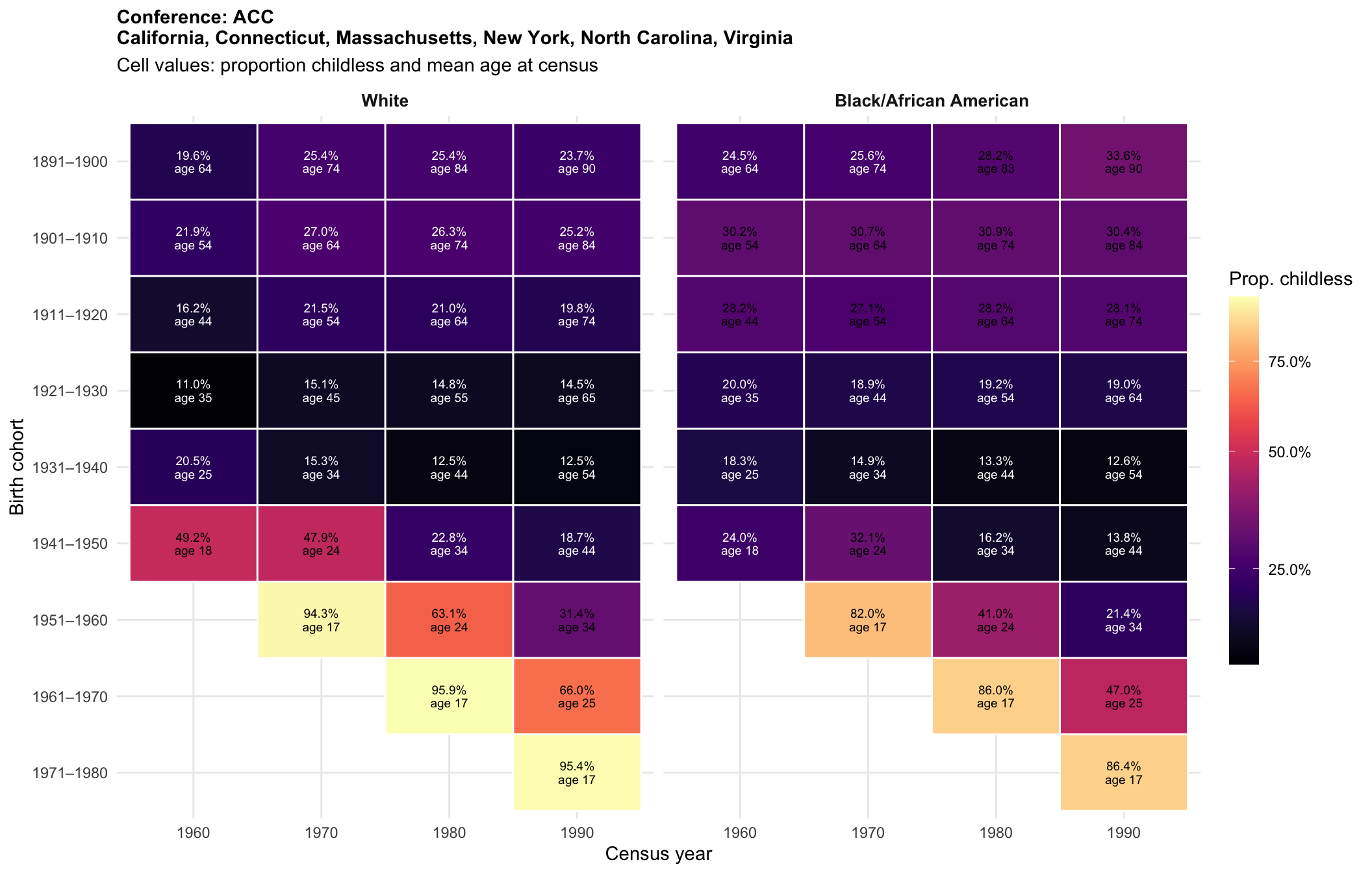
• ACC: California, Connecticut, Massachusetts, New York, North Carolina, Virginia
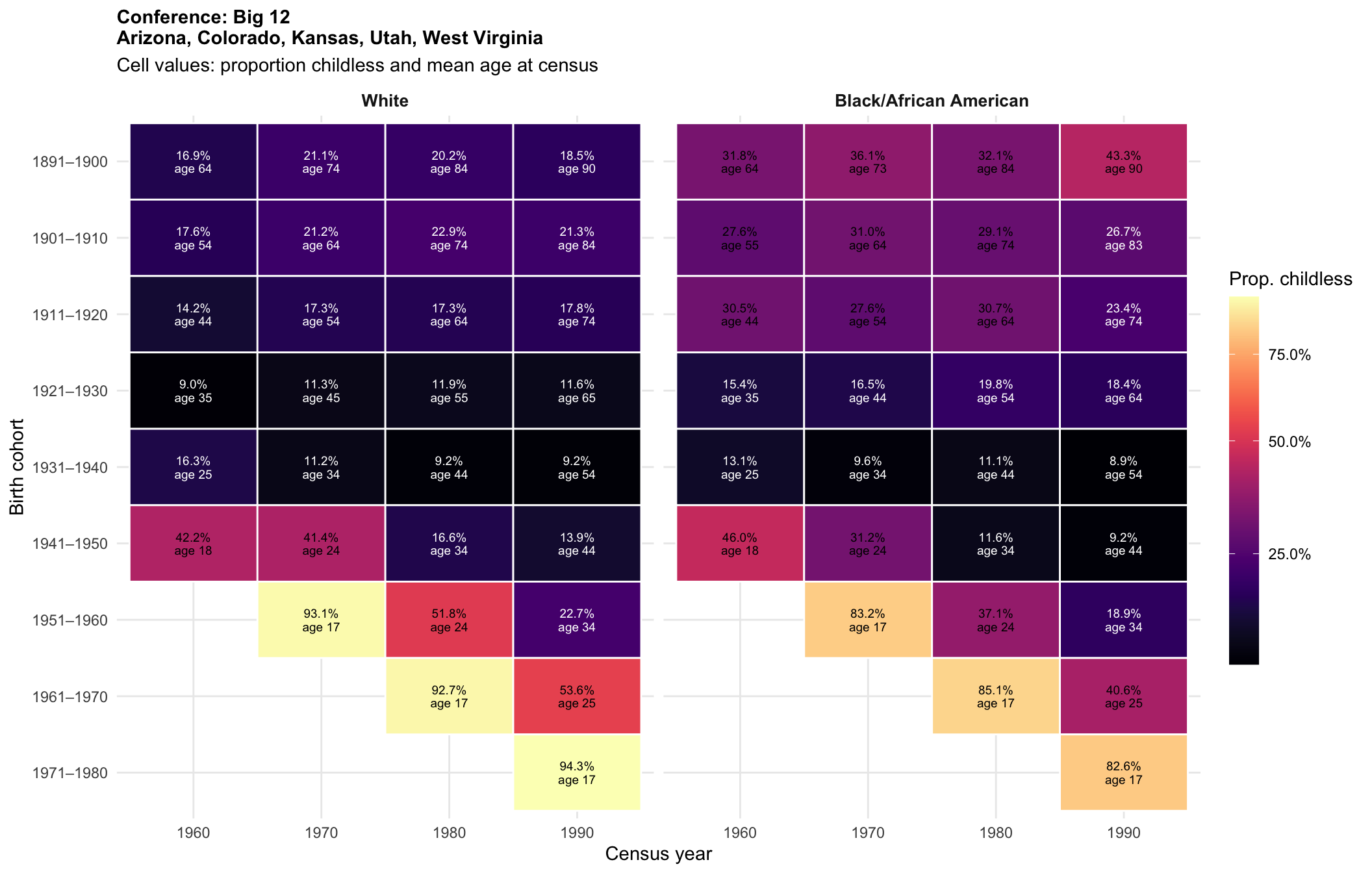
• Big 12: Arizona, Colorado, Kansas, Utah, West Virginia
• Other: Alaska, Delaware, Hawaii, Idaho, Maine, Montana, Nevada, New Hampshire, New Mexico, North Dakota, Rhode Island, South Dakota, Vermont, Wyoming, District of Columbia

data_with_conf <- data %>%
  mutate(conference = state_to_conference(state_name))

conf_cells <- data_with_conf %>%
  count(conference, RACE, YEAR, name = "n_obs") %>%
  filter(!is.na(conference))

conf_eligible <- conf_cells %>%
  filter(n_obs >= 30) %>%
  group_by(conference) %>%
  filter(all(c("White", "Black/African American") %in% RACE)) %>%
  pull(conference) %>%
  unique() %>%
  sort()

cat(length(conf_eligible), "conferences with adequate data:\n")

5 conferences with adequate data:

cat(paste(conf_eligible, collapse = ", "), "\n")

ACC, Big 12, Big Ten, Other, SEC 

for (conf in conf_eligible) {
  conf_data <- data_with_conf %>%
    filter(conference == conf) %>%
    mutate(chborn_capped = pmin(chborn_num, 12))

  if (n_distinct(conf_data$RACE) < 2) next

  states_in_conf <- sort(unique(conf_data$state_name))
  plot_title <- paste0("Conference: ", conf, "\n",
                       str_wrap(paste(states_in_conf, collapse = ", "), width = 80))
  p <- plot_state_fertility(conf_data, plot_title)
  print(p)
  cat("\n\n")
}

Past versions of conference-plots-1.png

Version	Author	Date
9d44b29	Tina Lasisi	2026-04-14

Past versions of conference-plots-2.png

Version	Author	Date
9d44b29	Tina Lasisi	2026-04-14

Past versions of conference-plots-3.png

Version	Author	Date
9d44b29	Tina Lasisi	2026-04-14

Past versions of conference-plots-4.png

Version	Author	Date
9d44b29	Tina Lasisi	2026-04-14

Past versions of conference-plots-5.png

Version	Author	Date
9d44b29	Tina Lasisi	2026-04-14

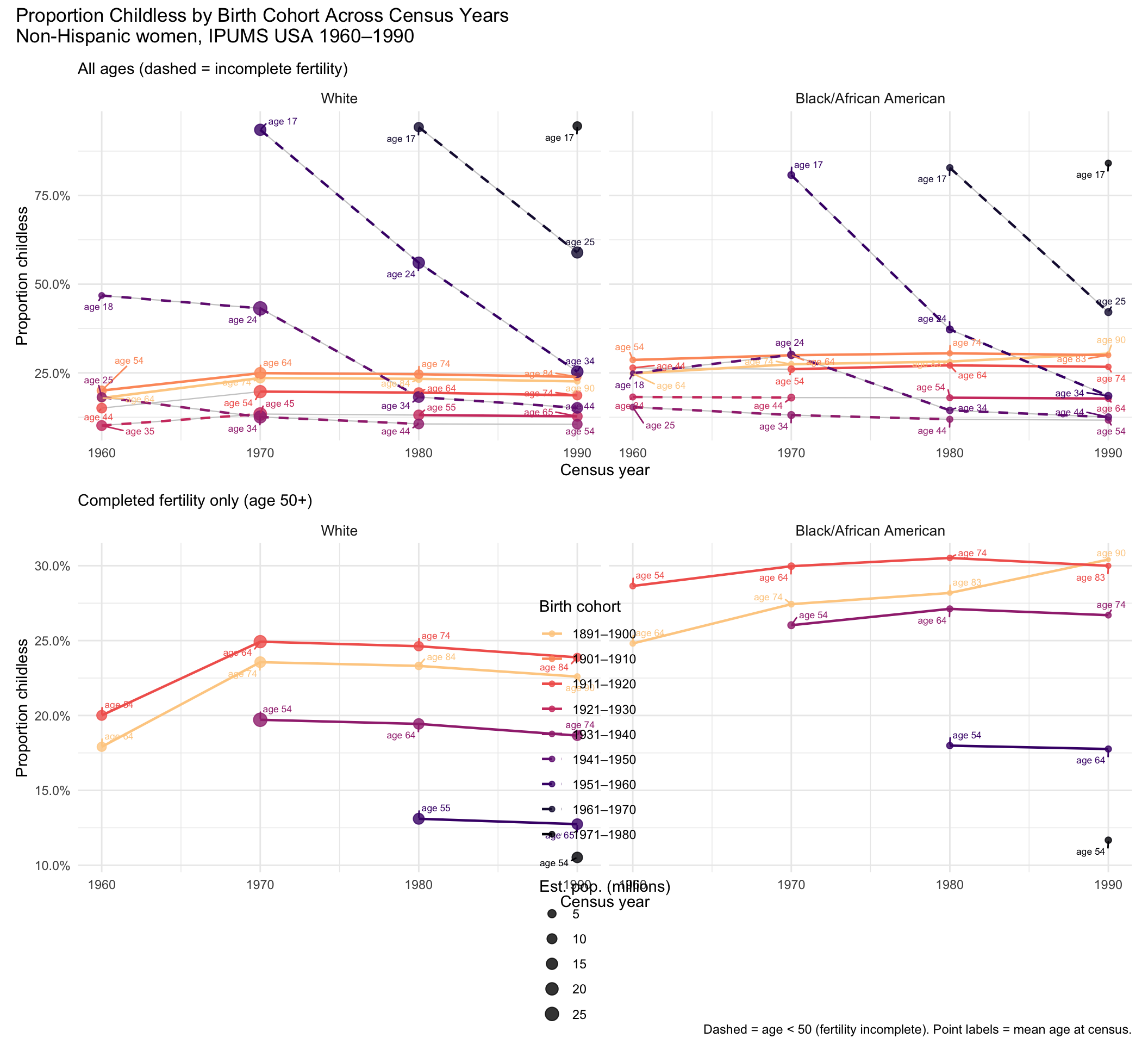
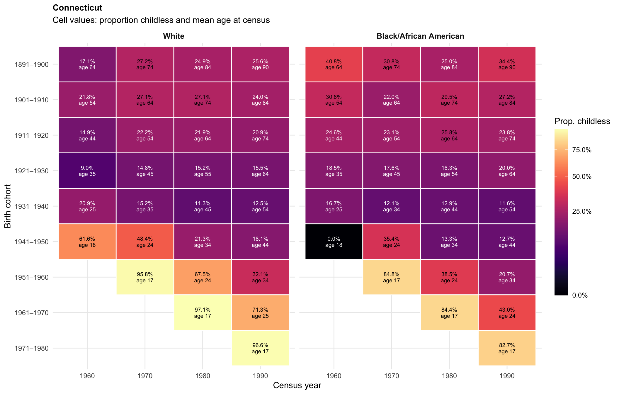
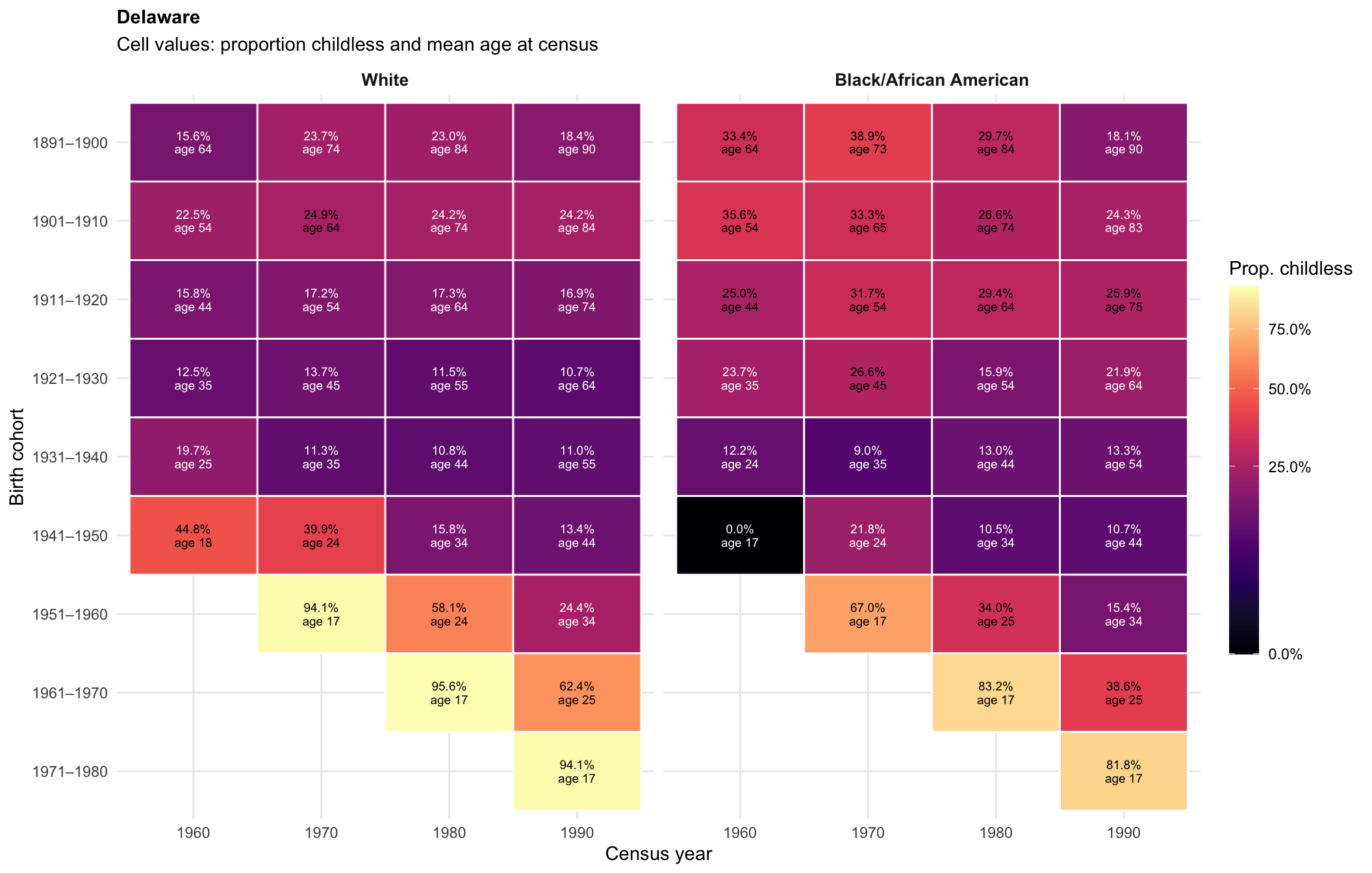
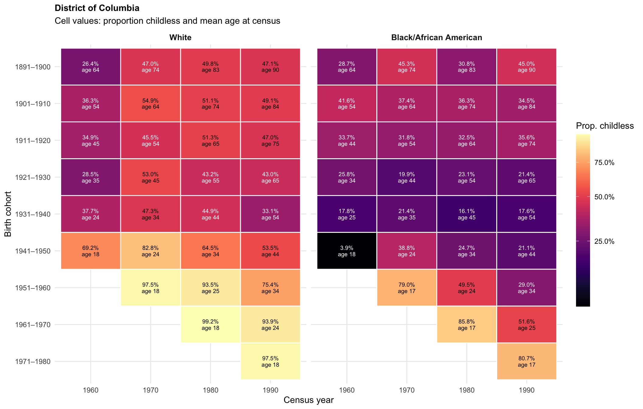
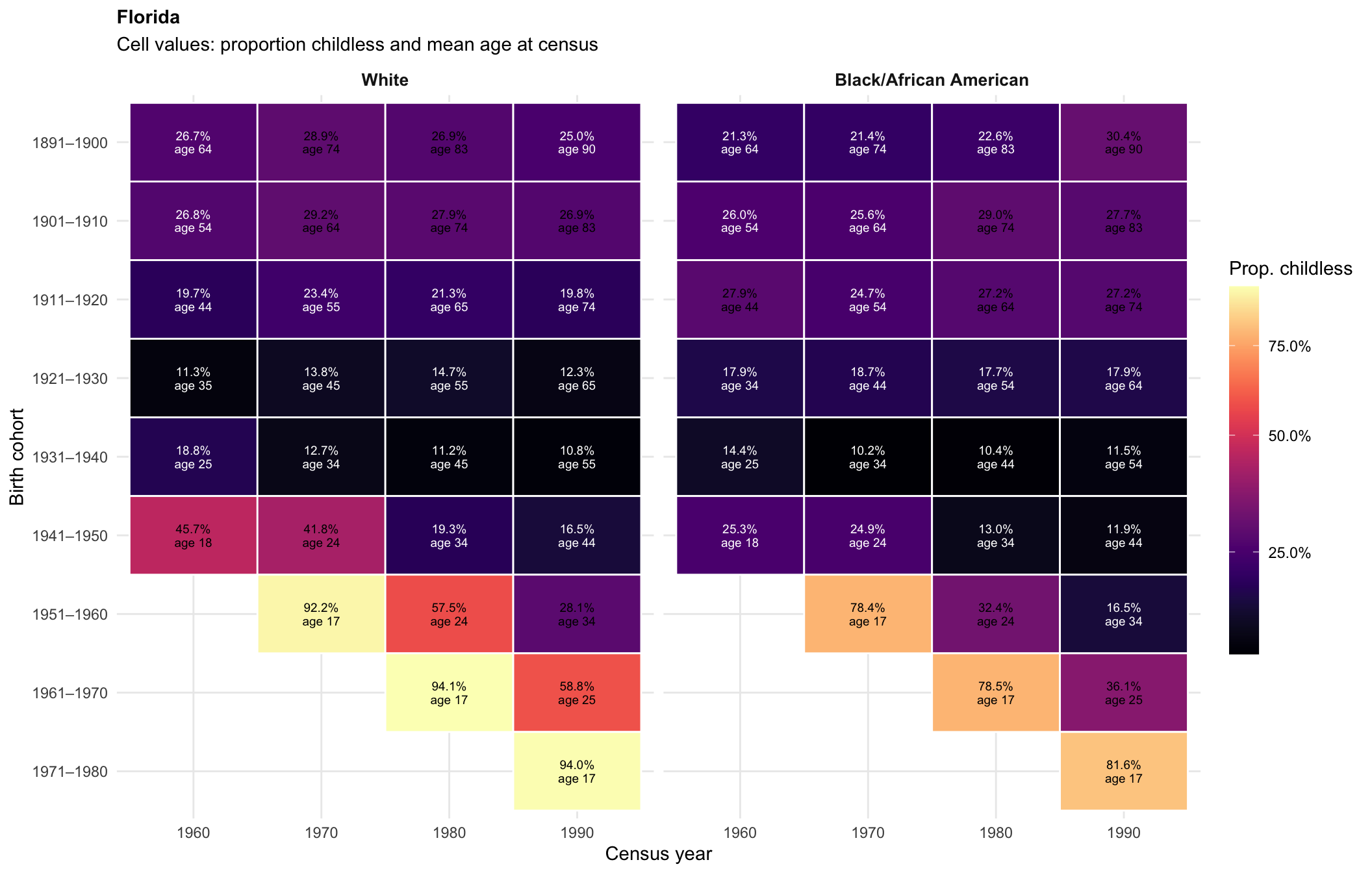
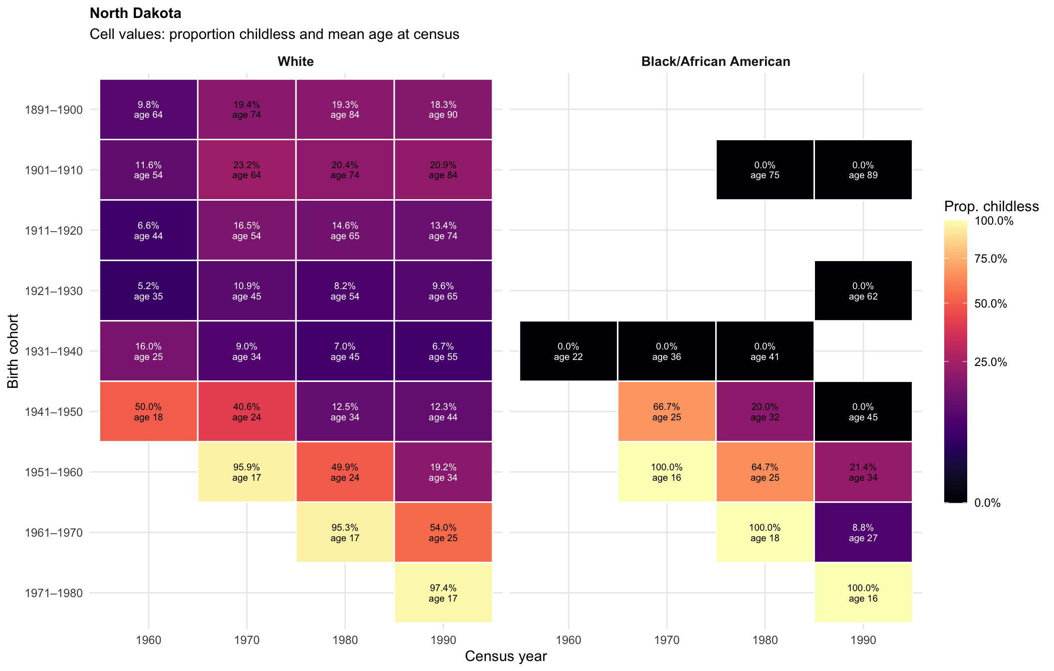
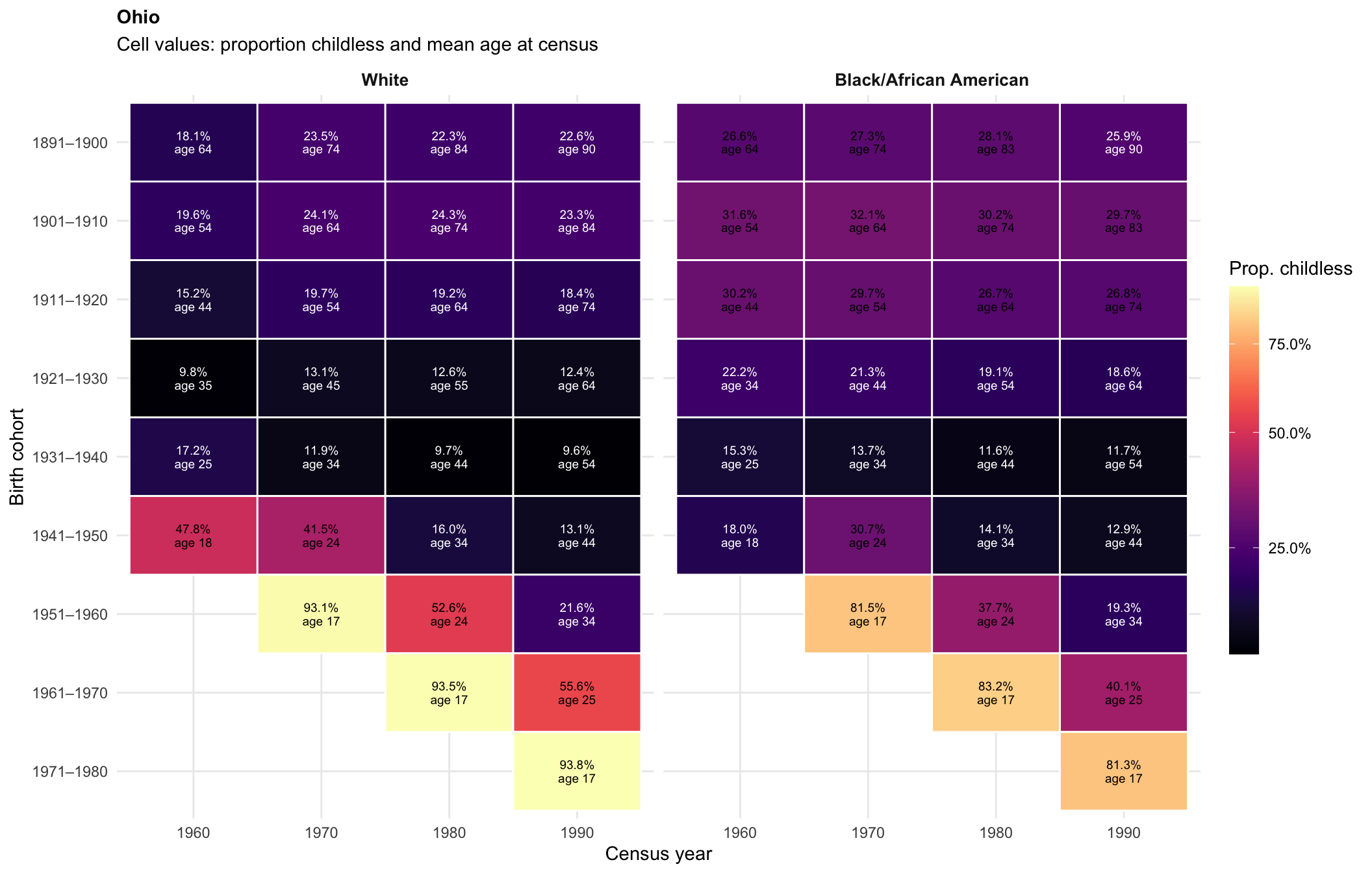
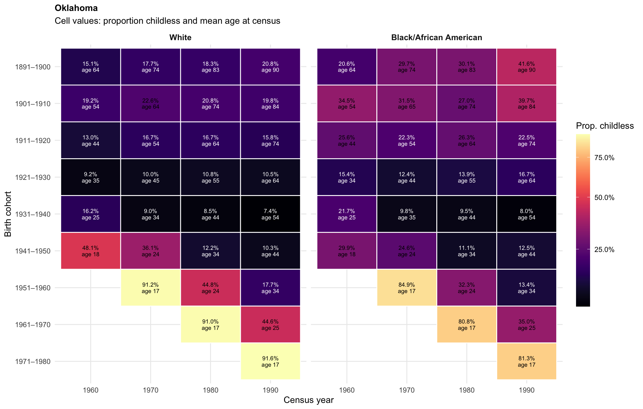
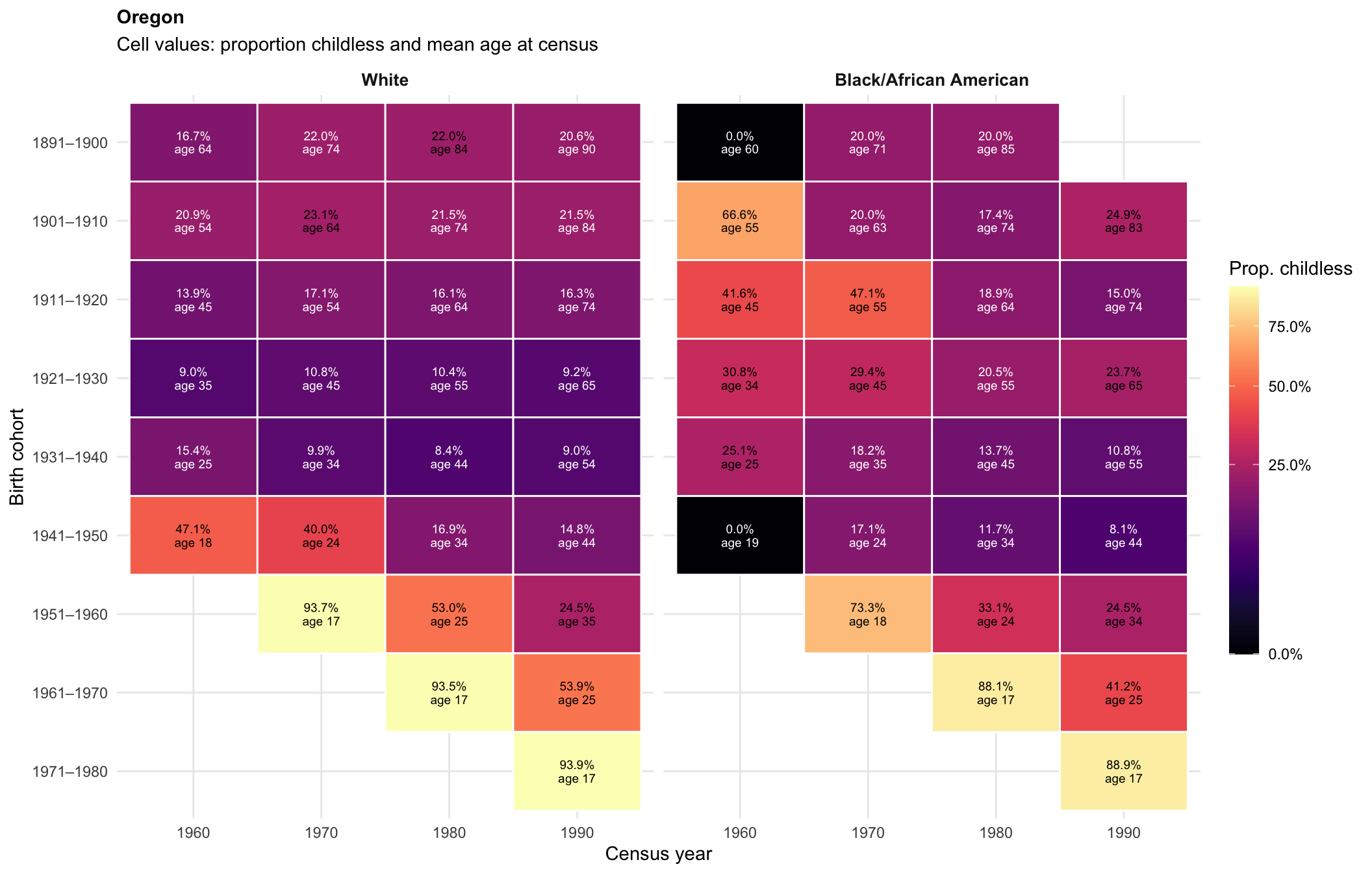
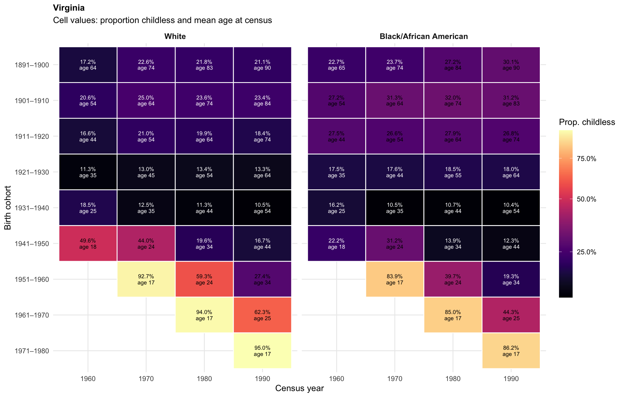
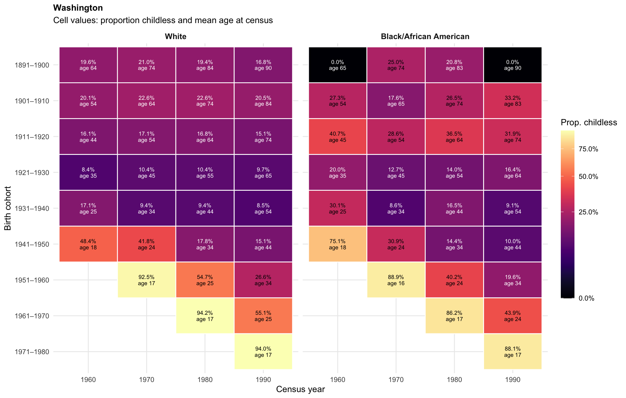
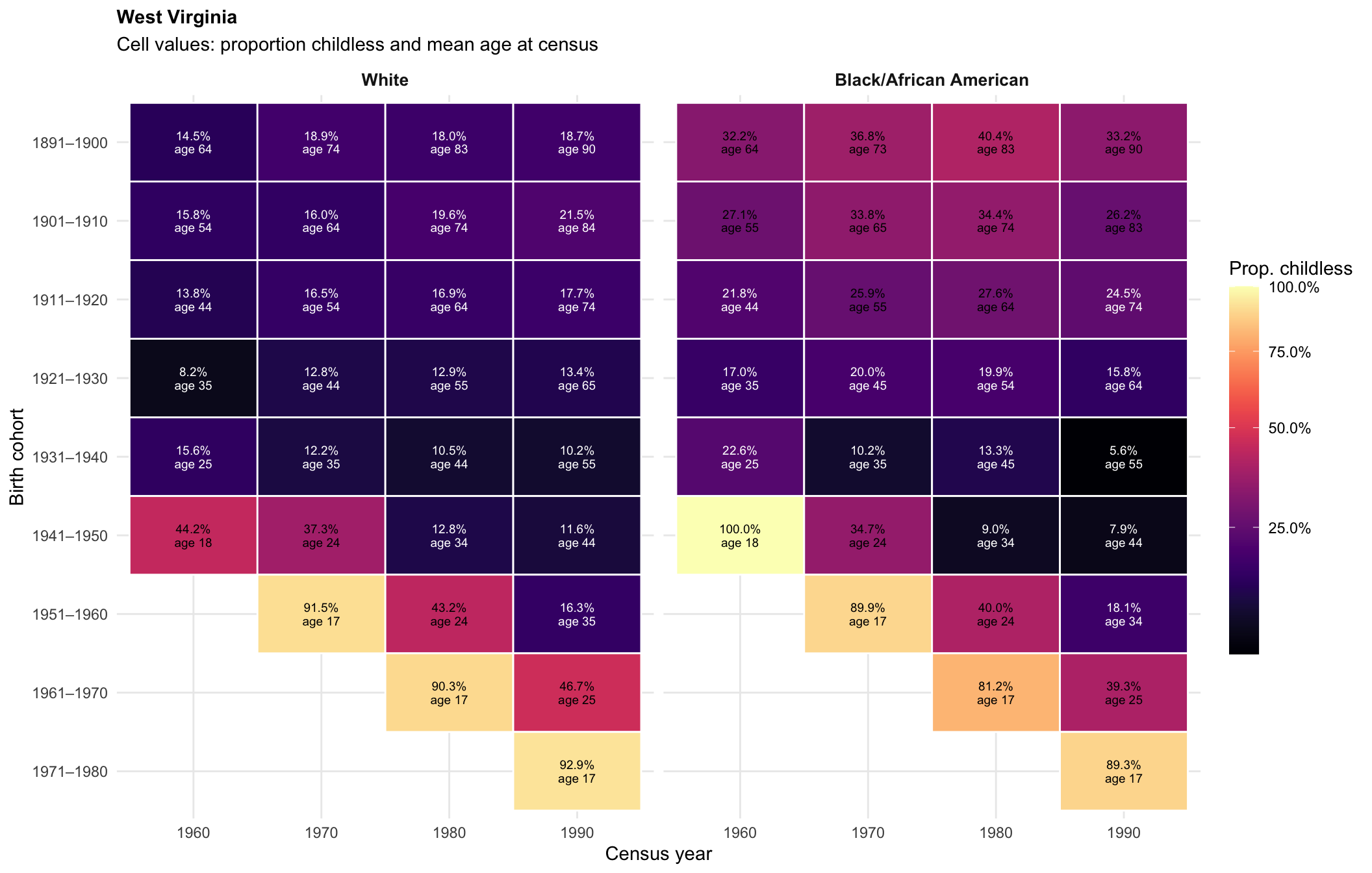
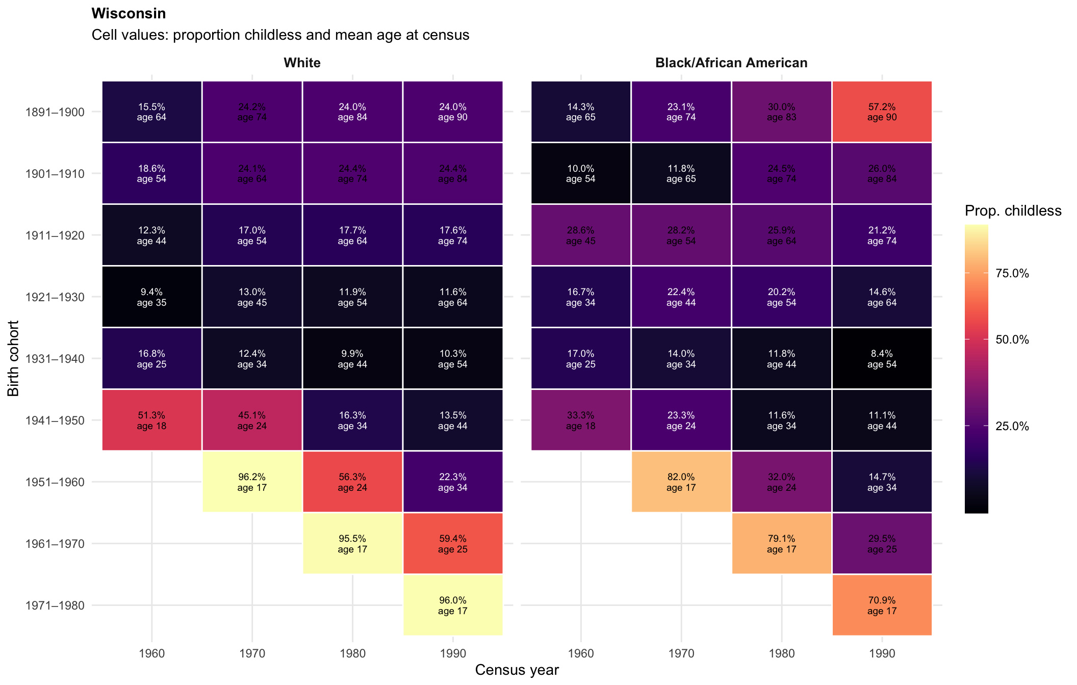
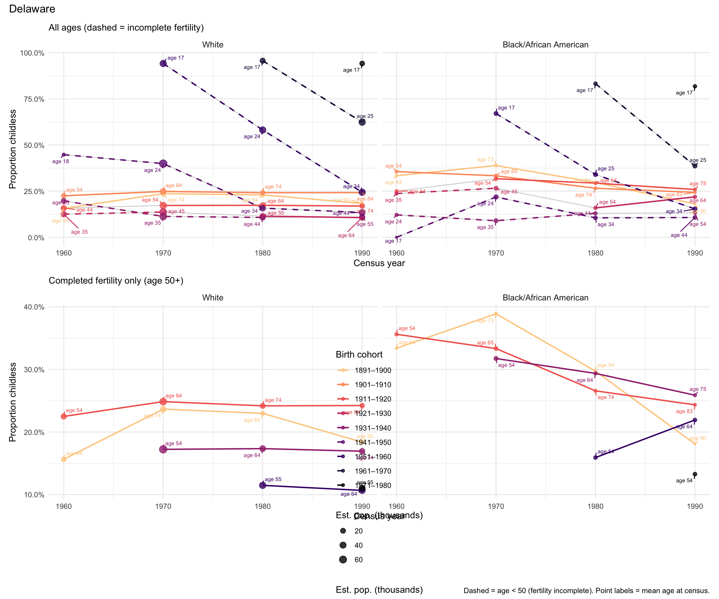
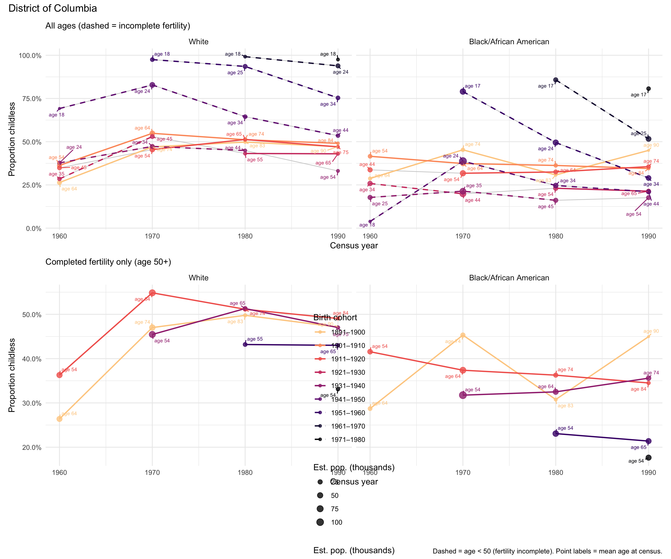
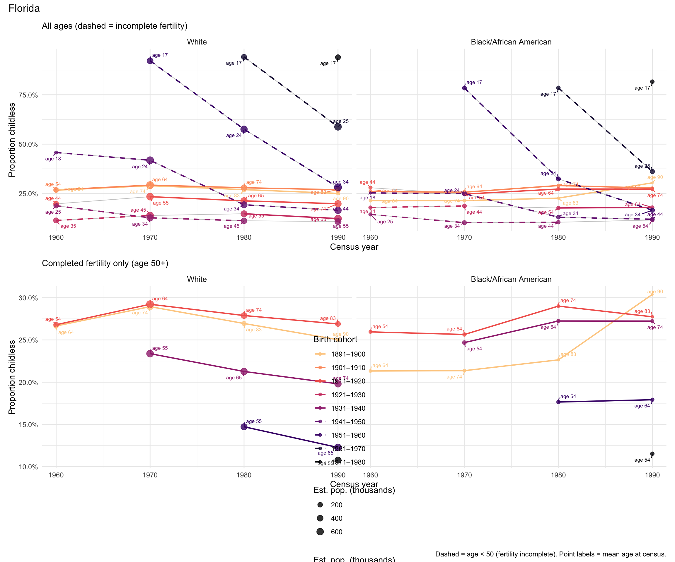
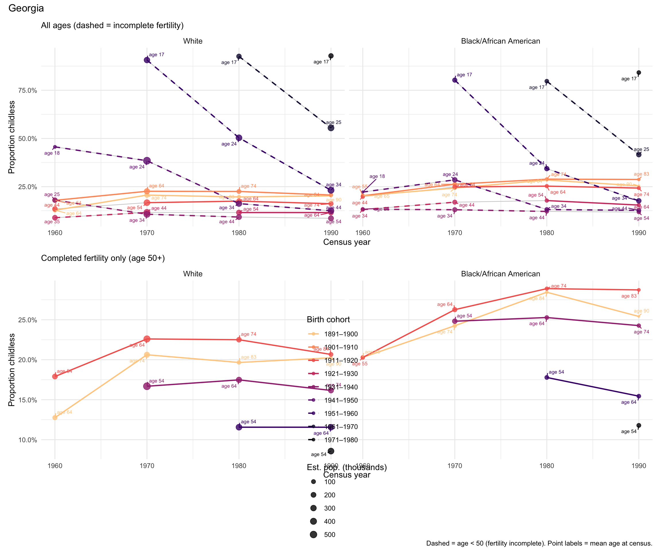
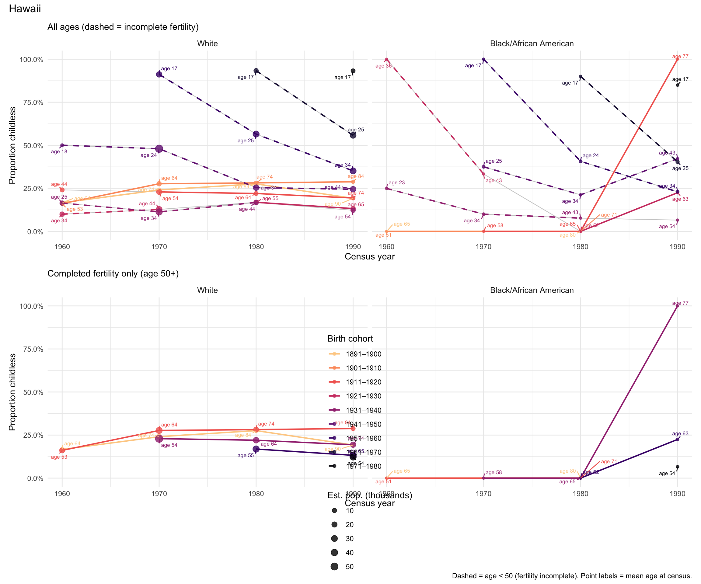
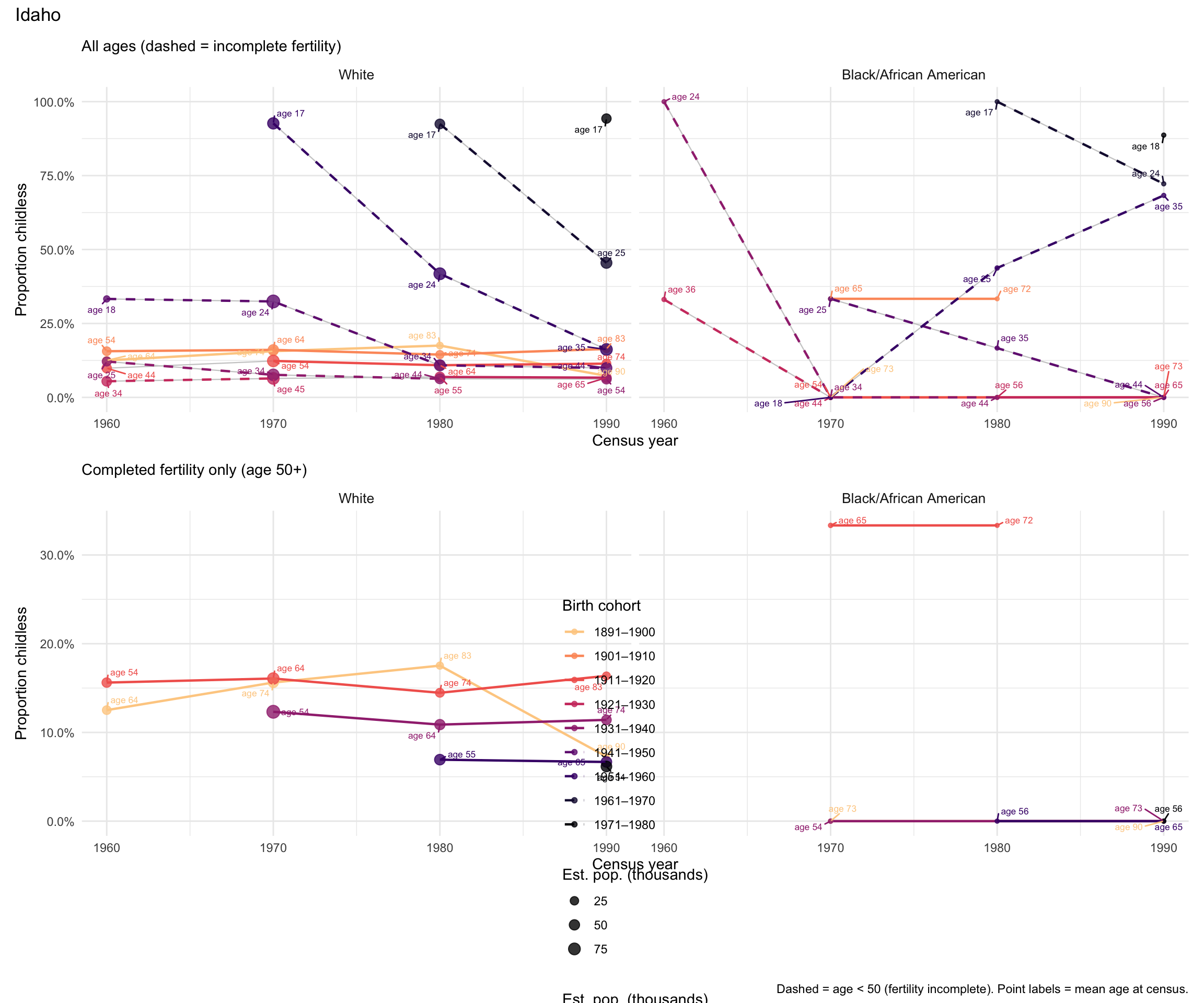
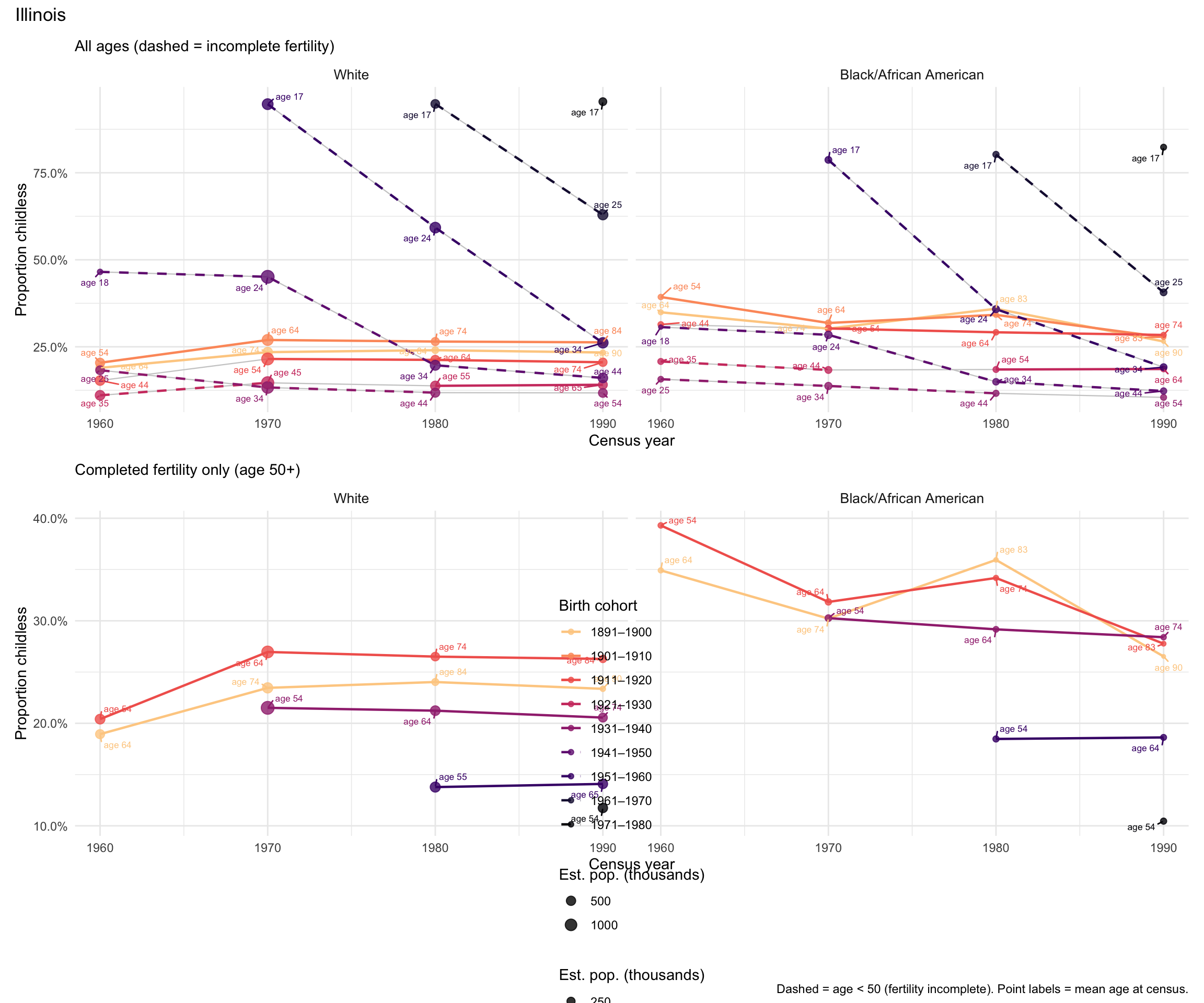
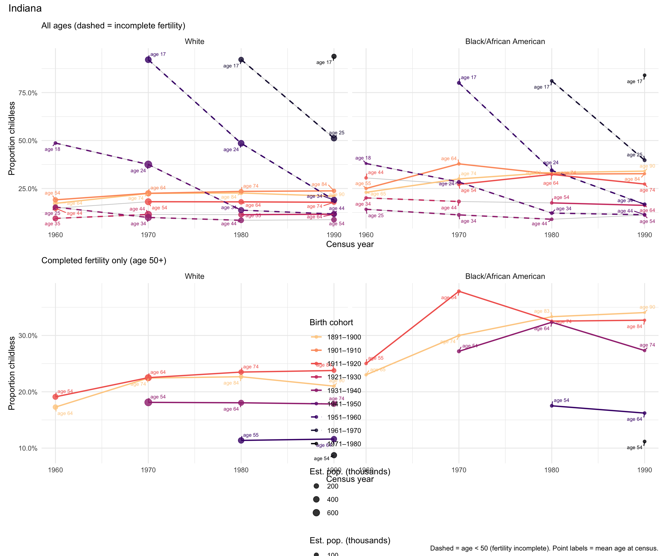
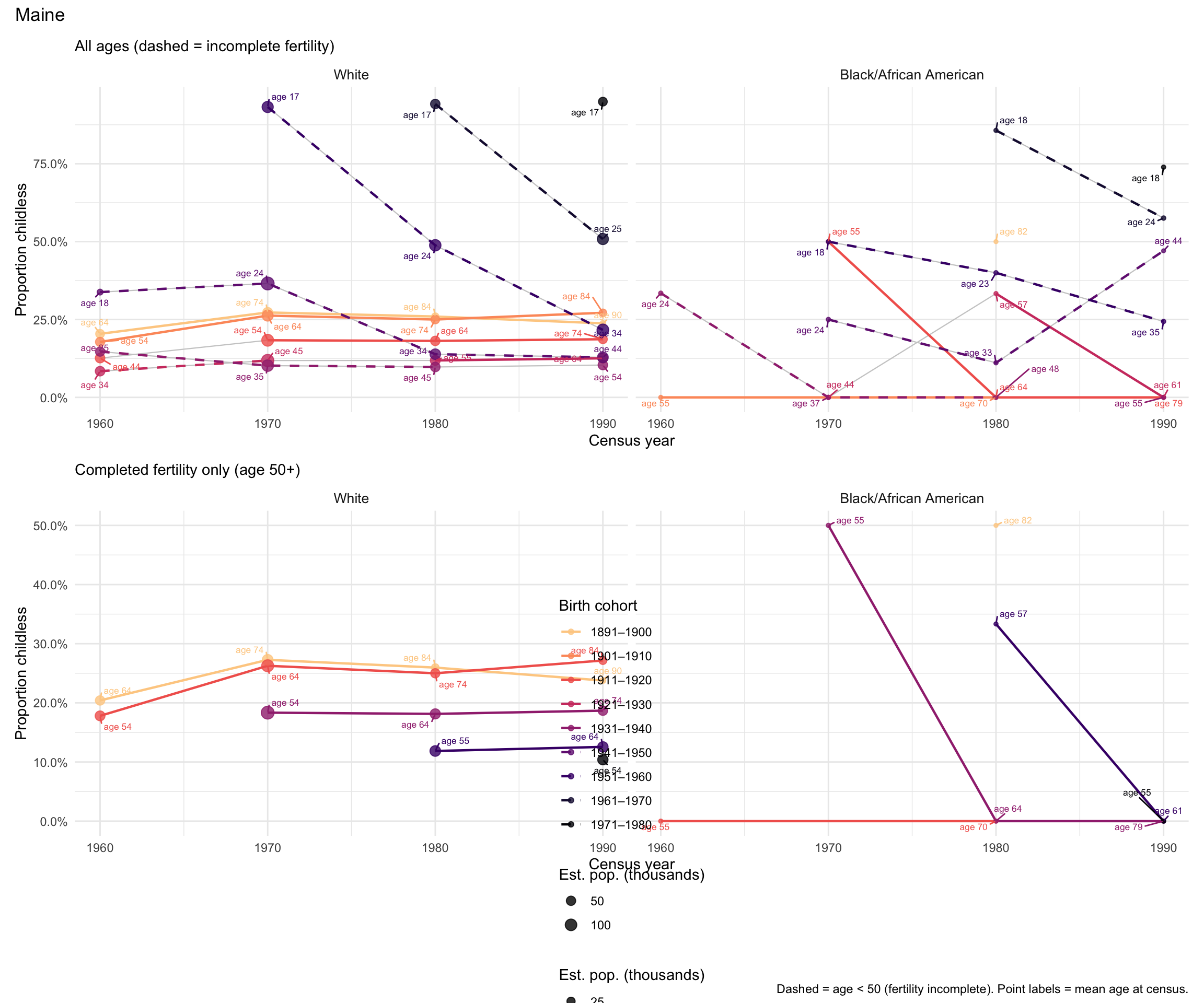
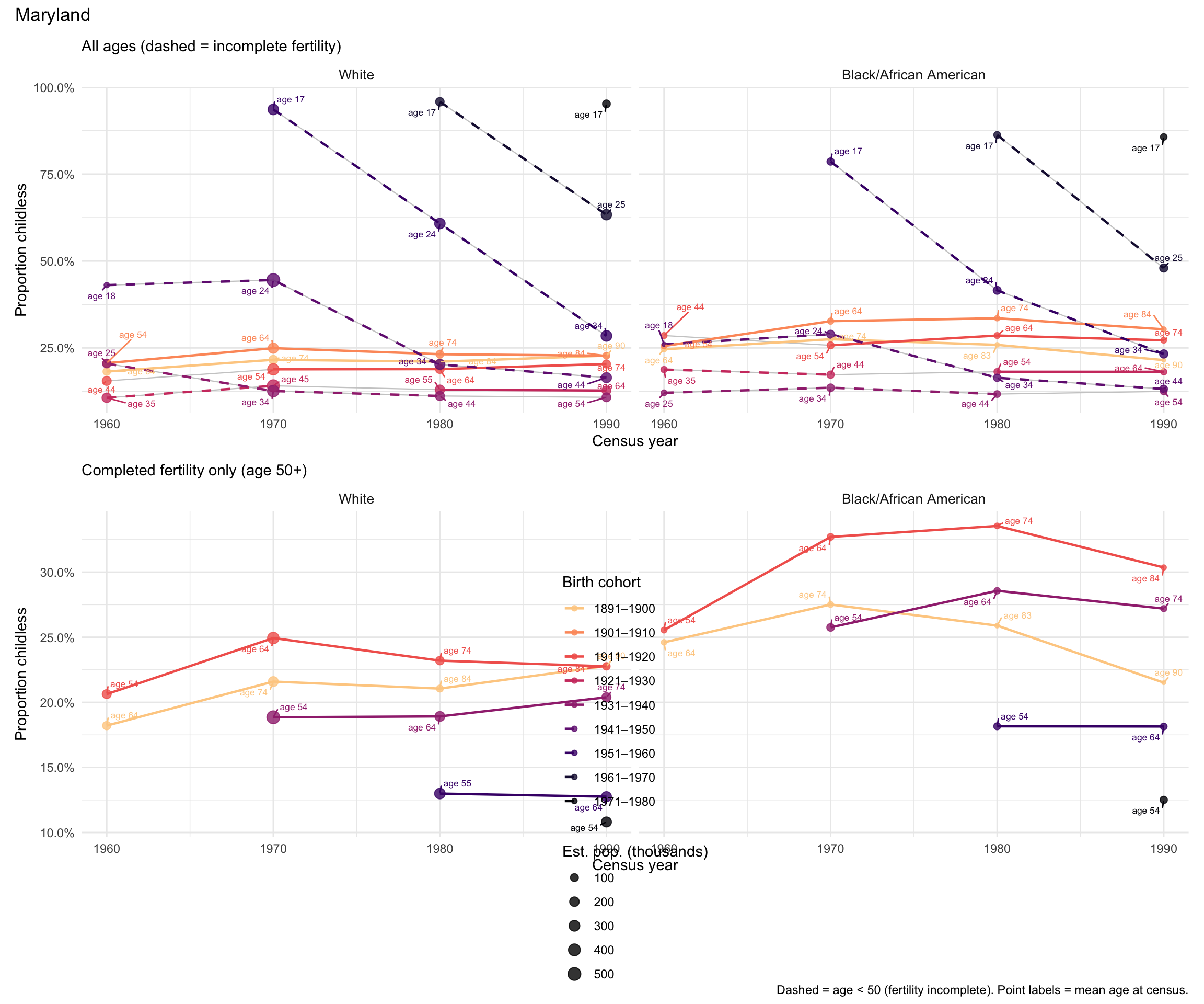
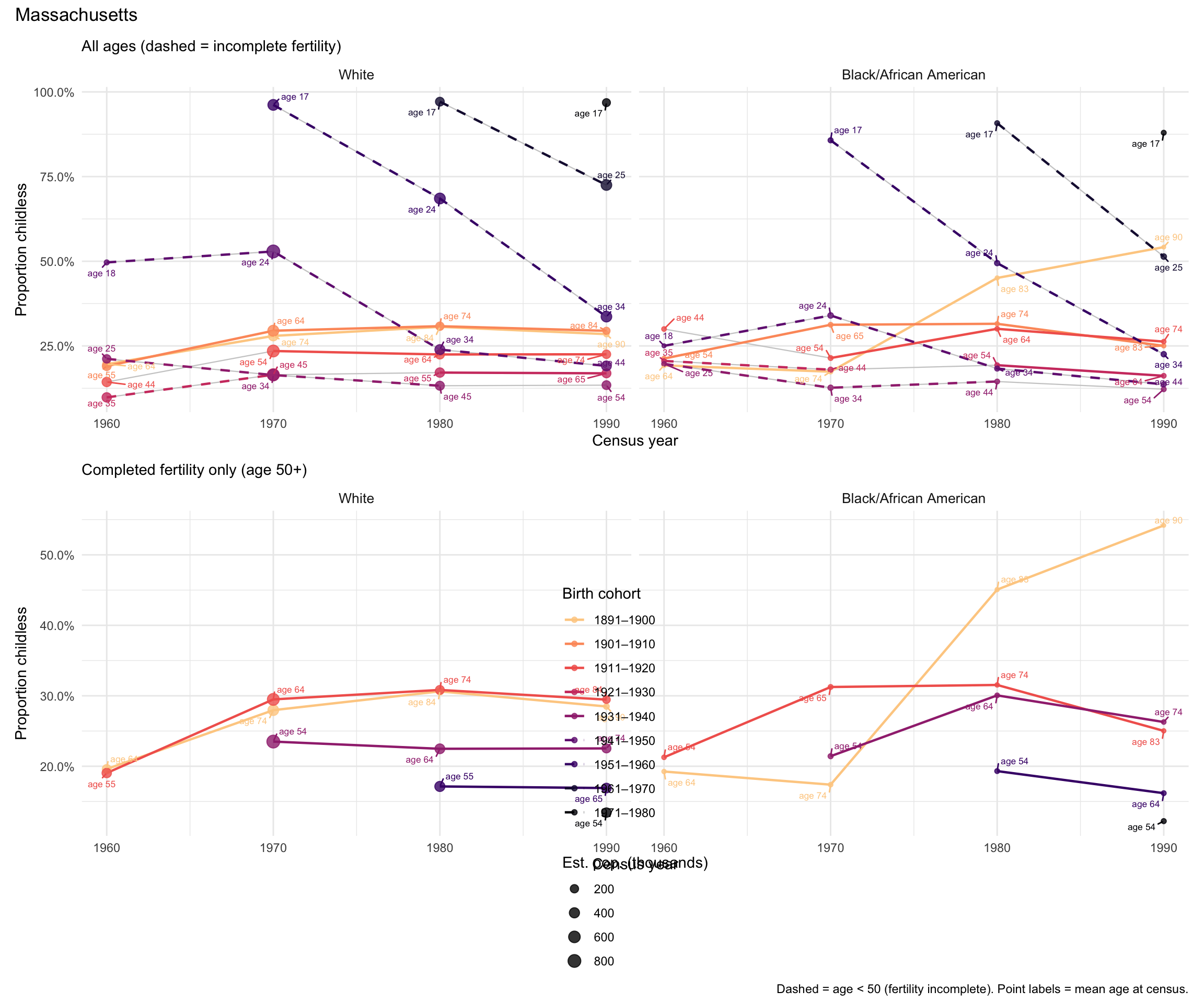
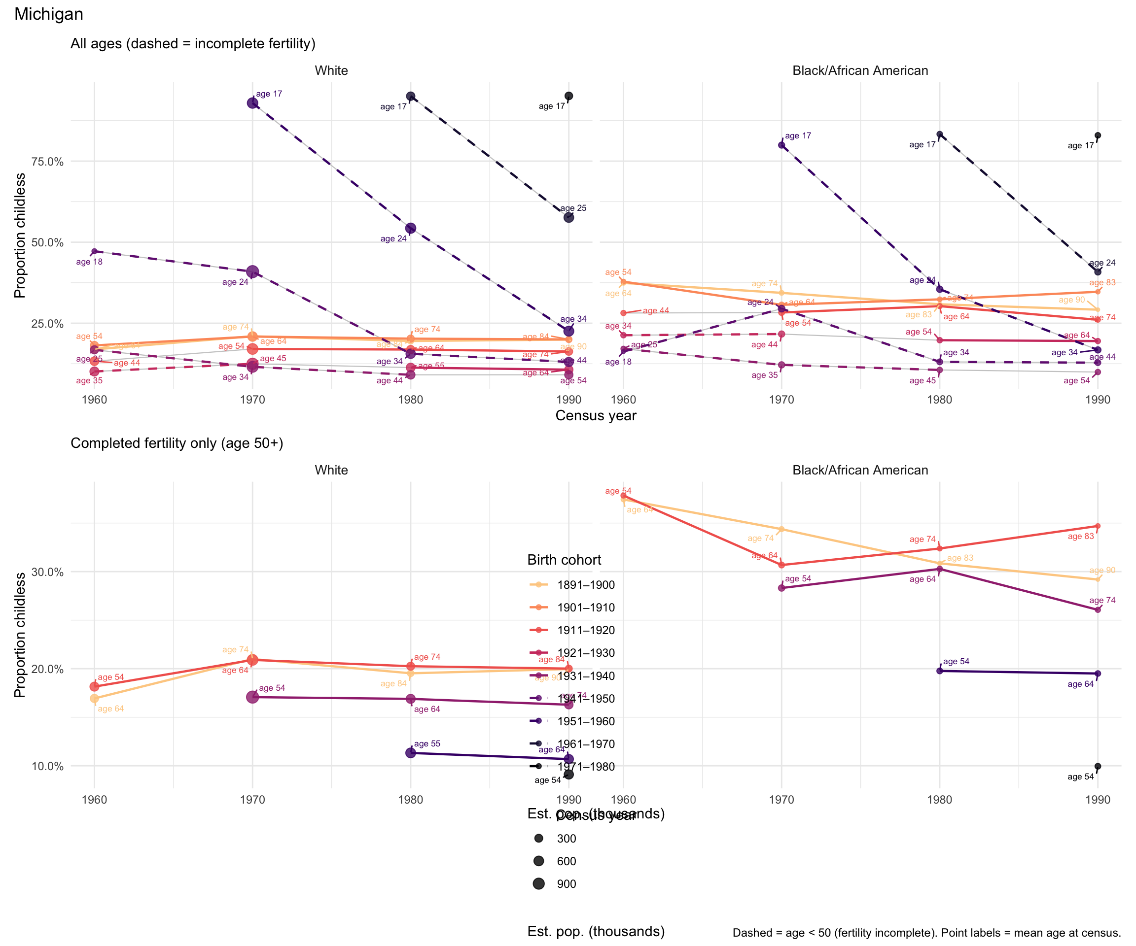
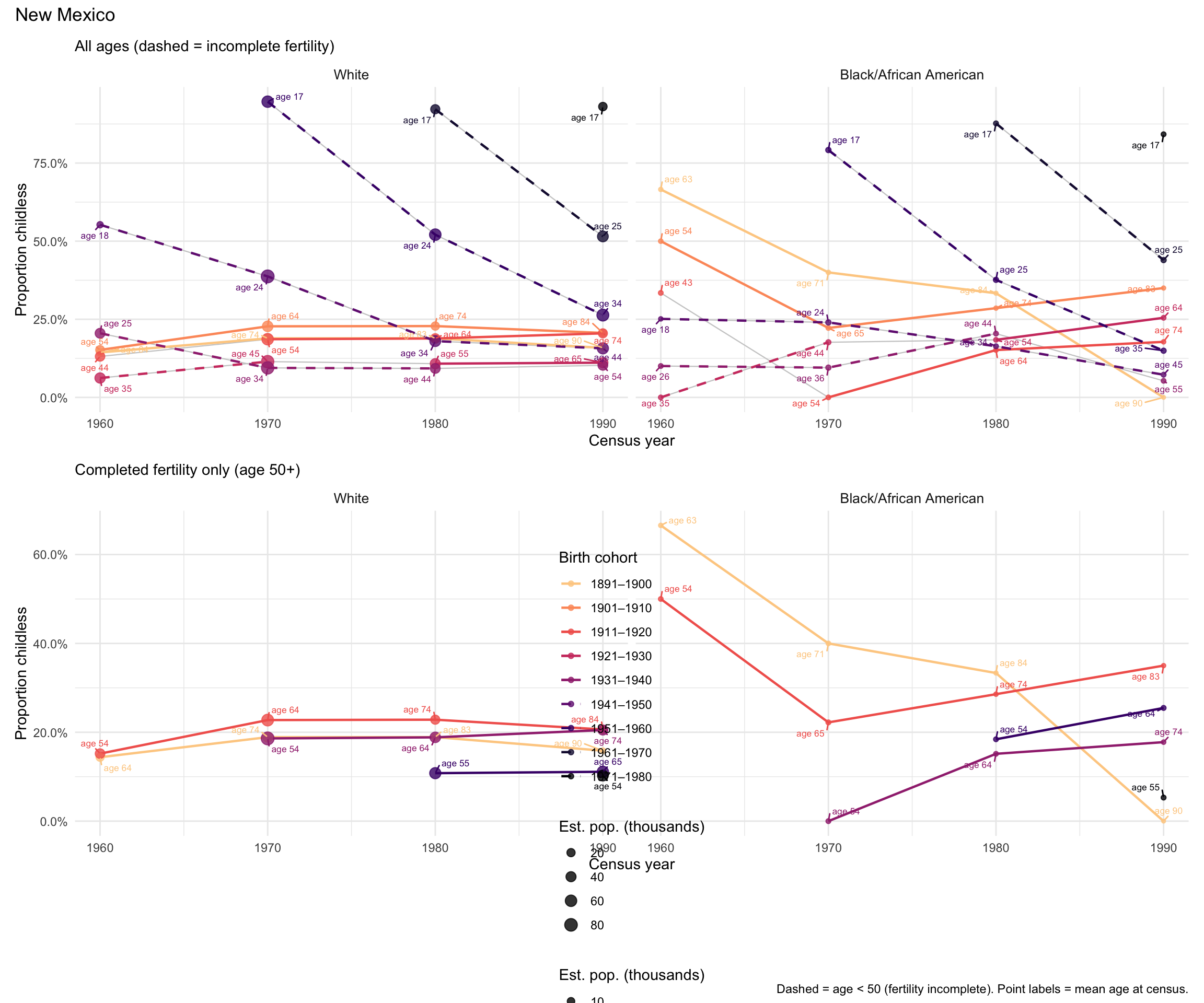
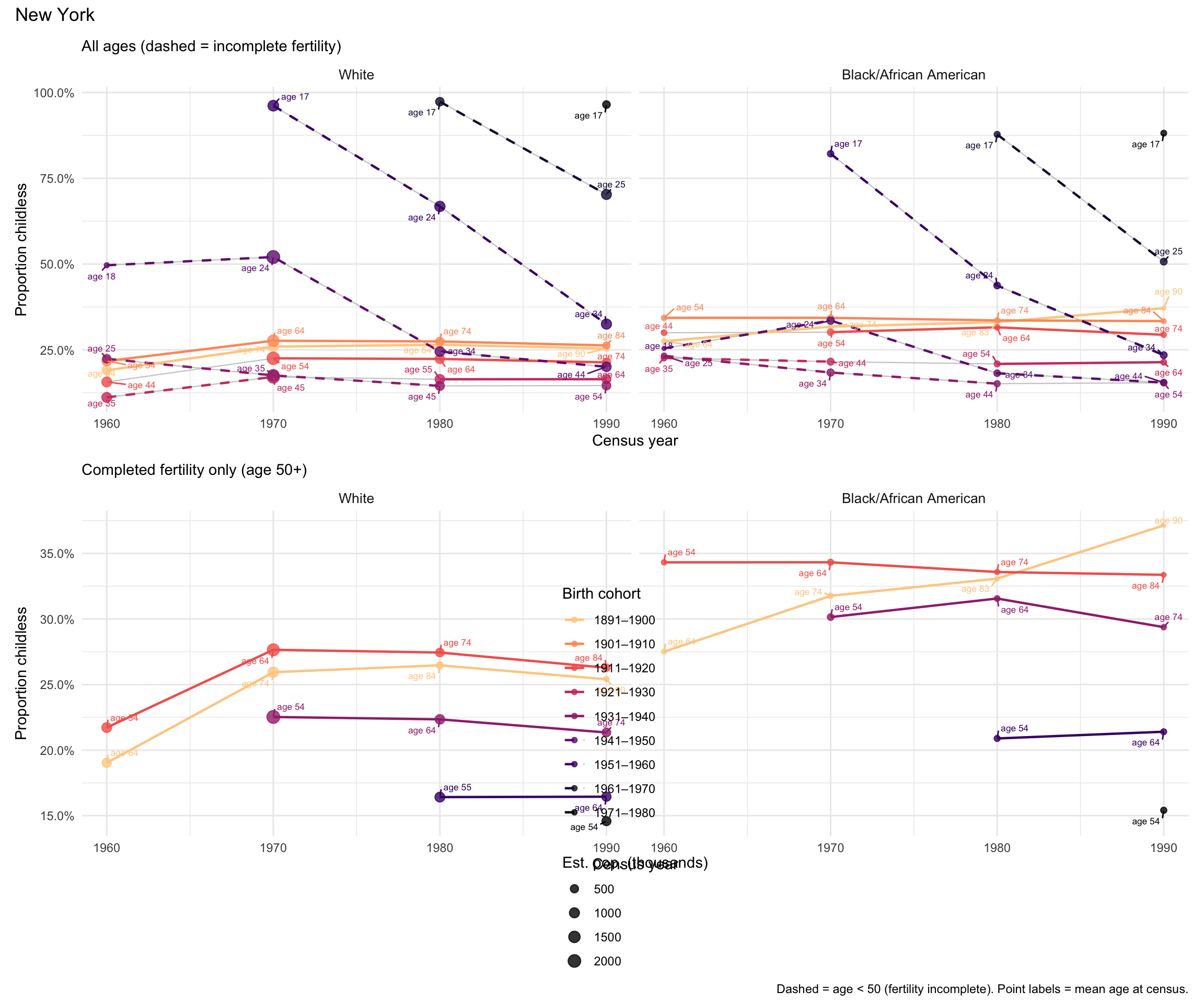
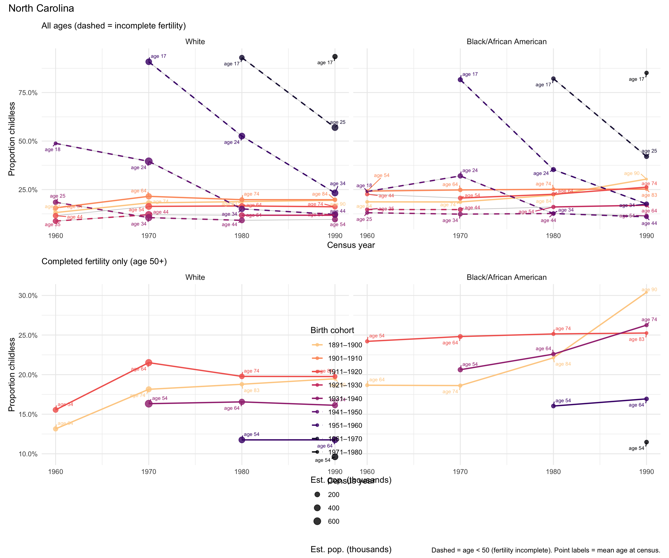
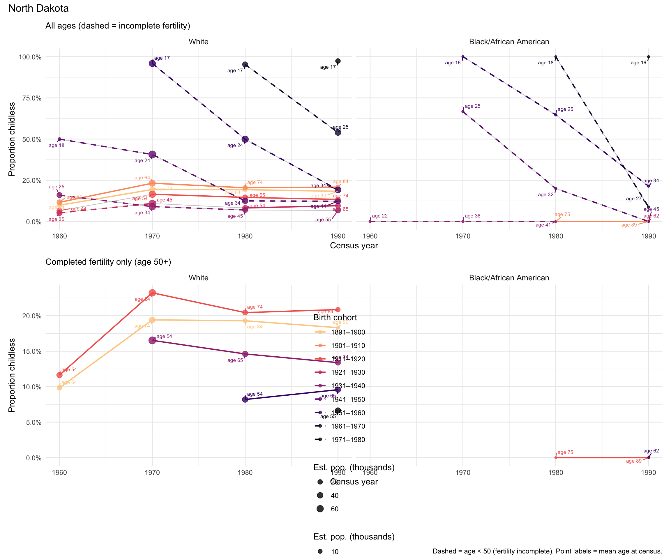
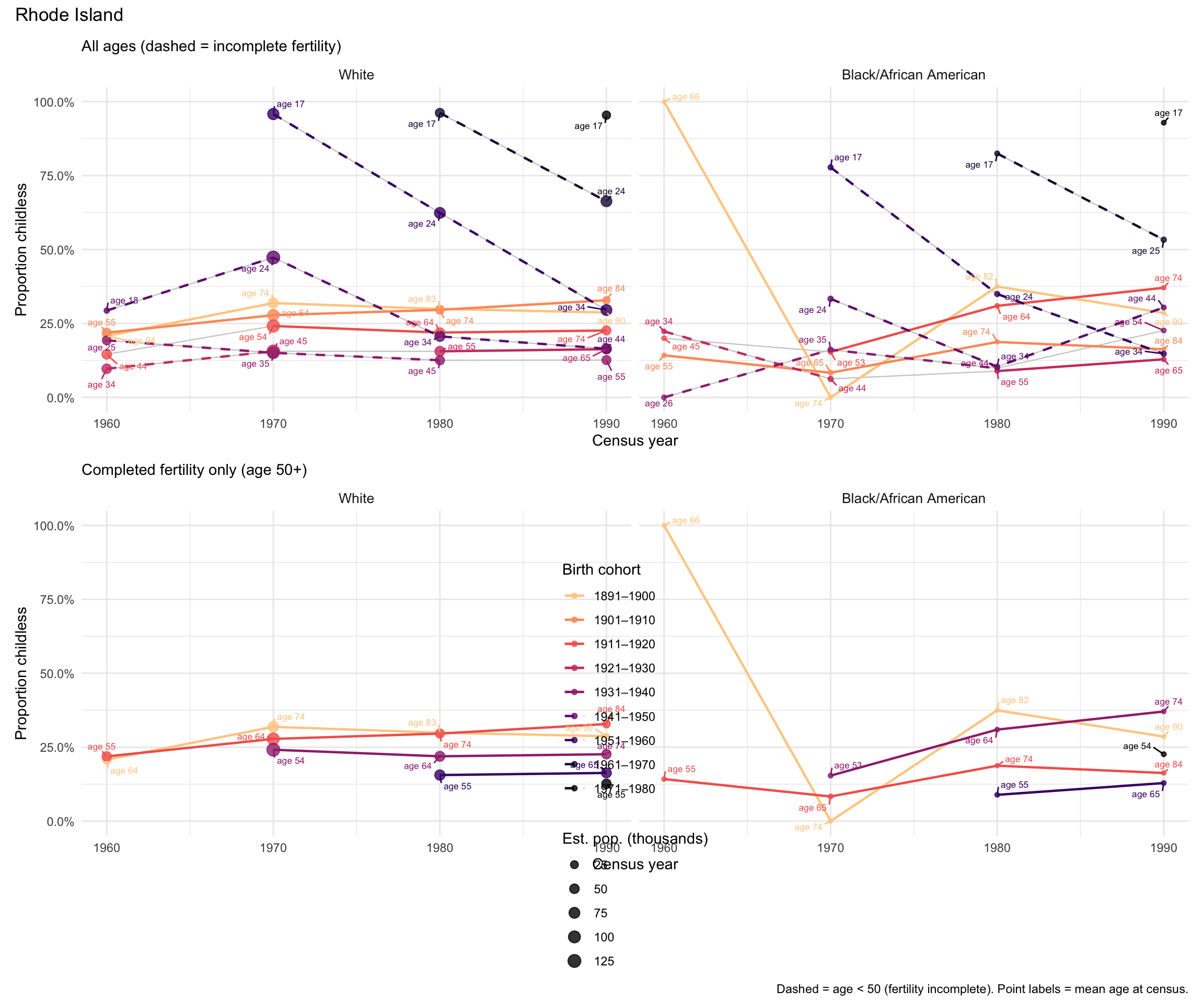
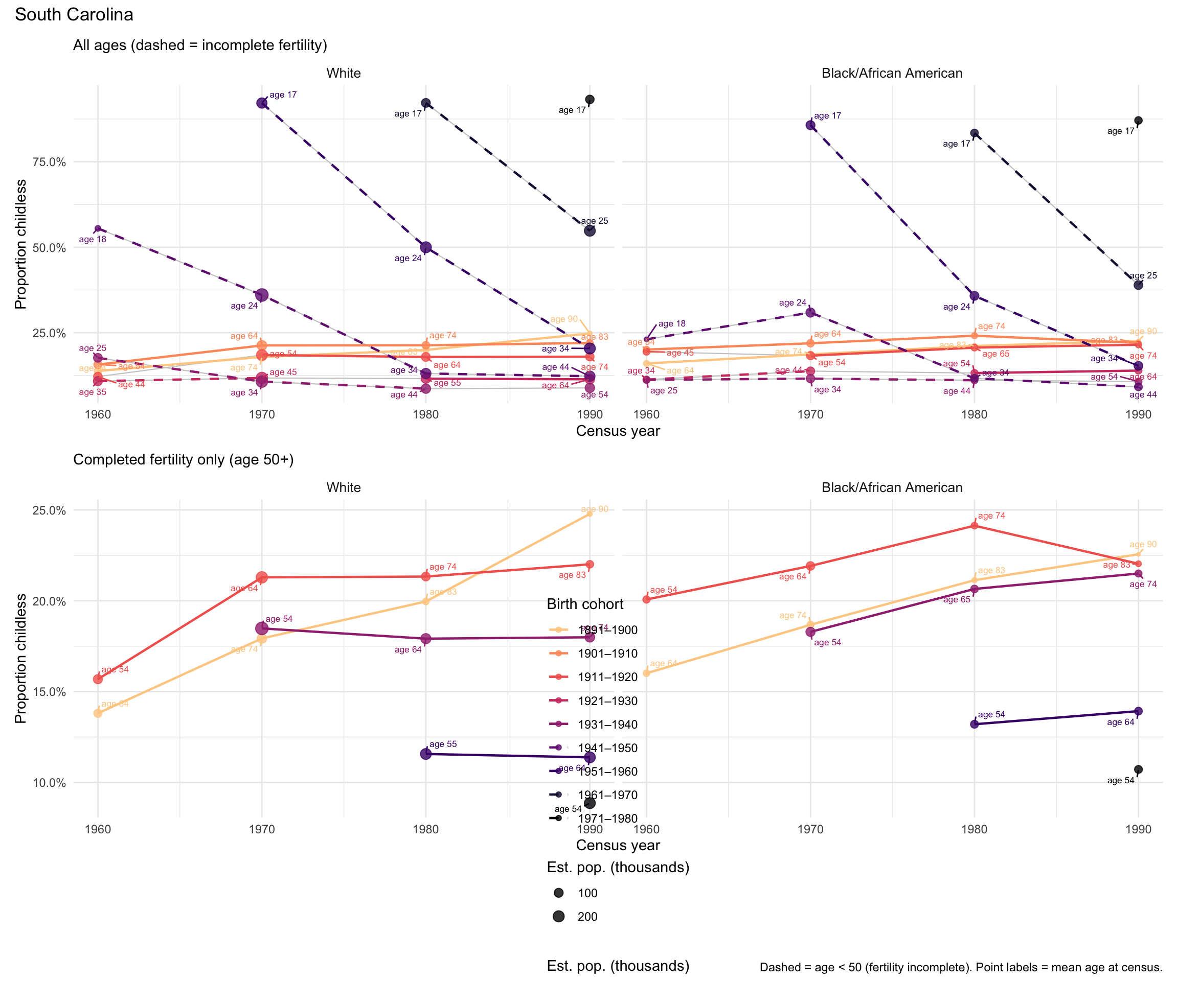
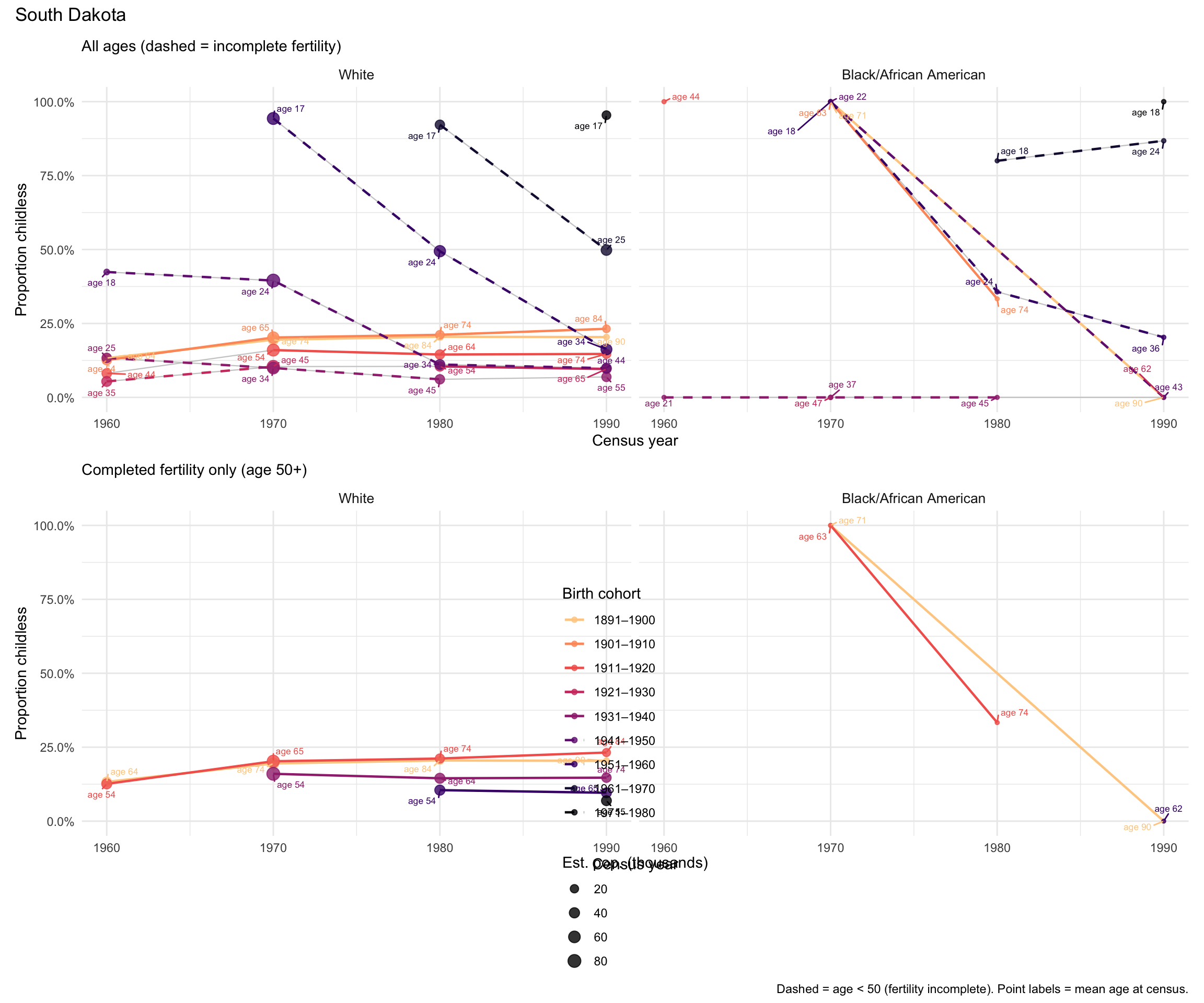
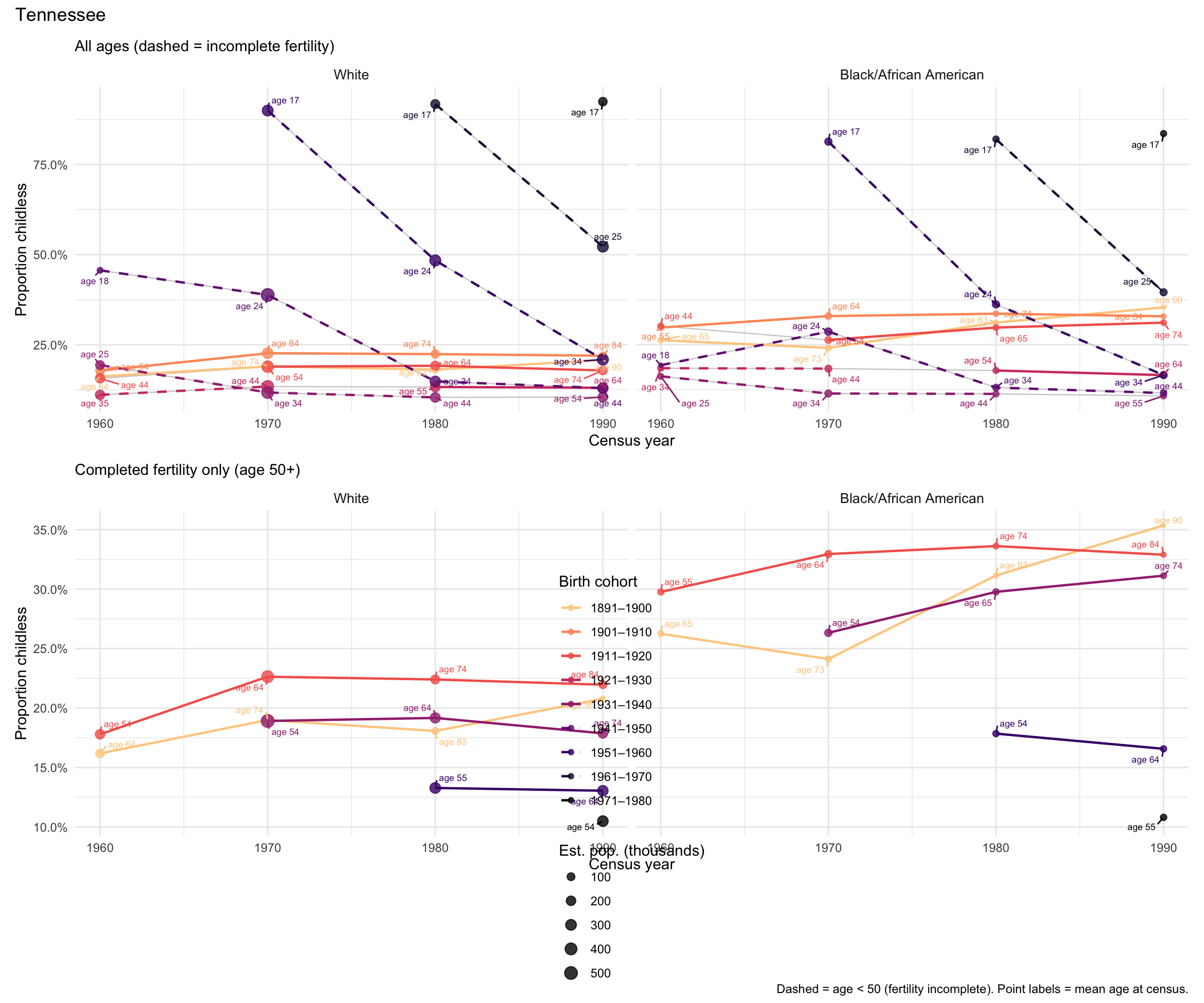
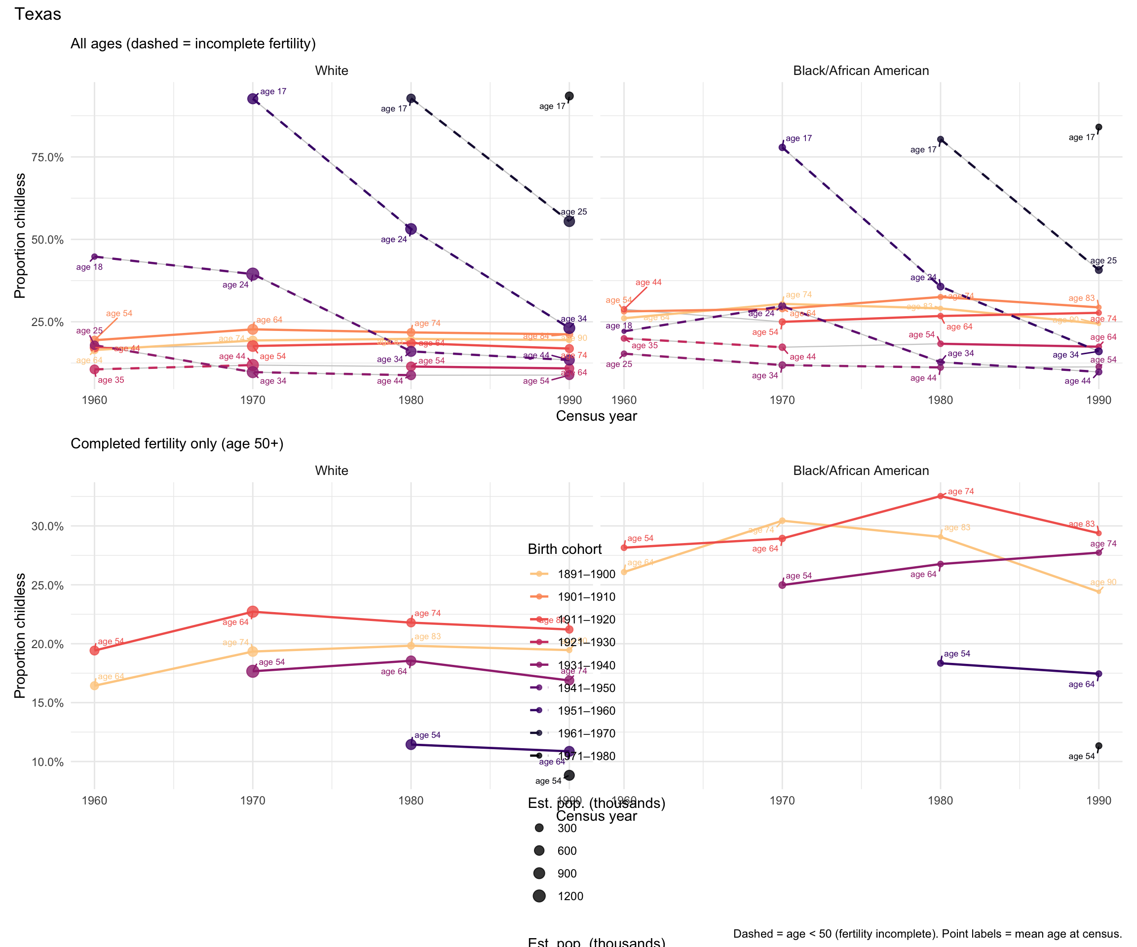
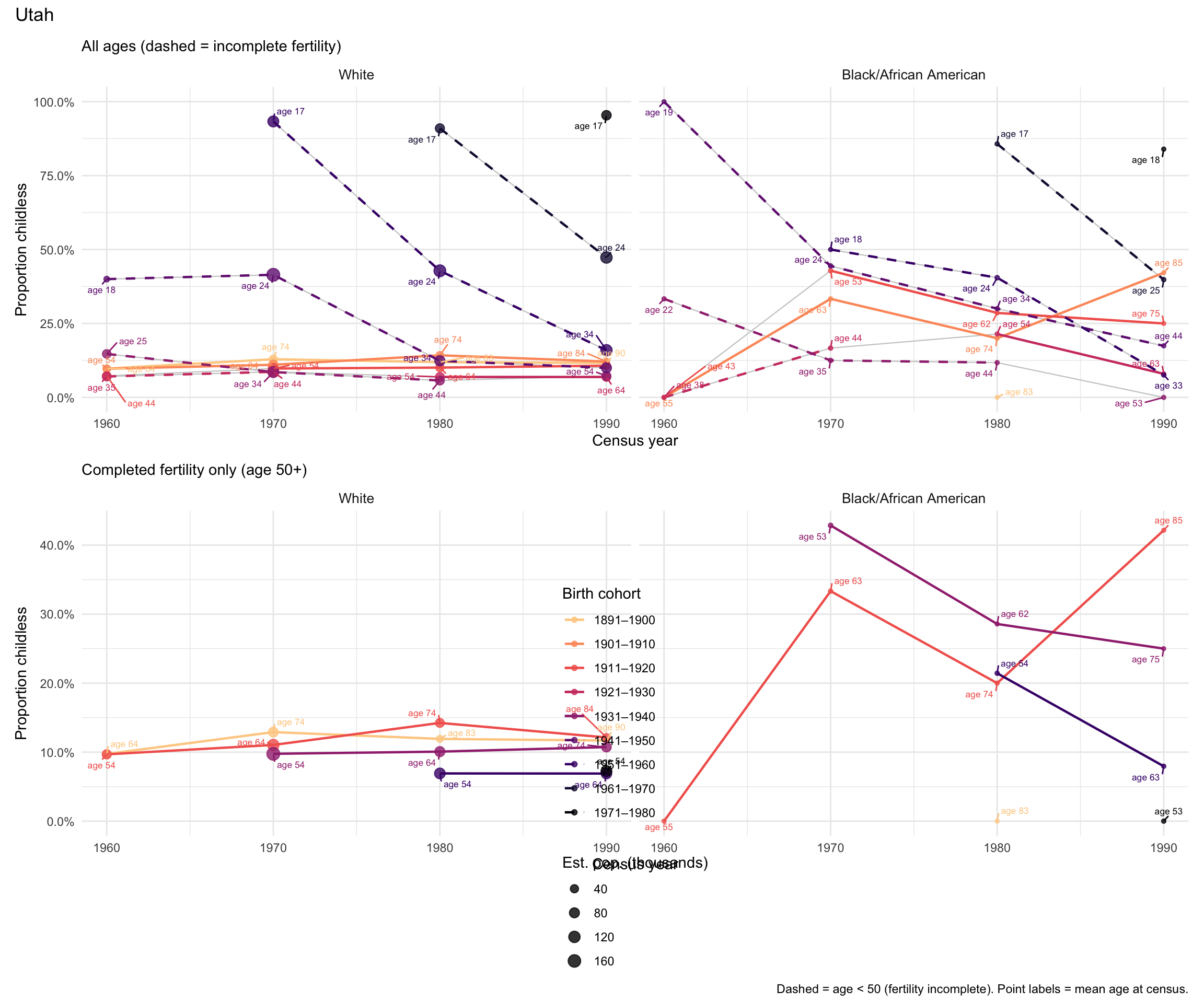
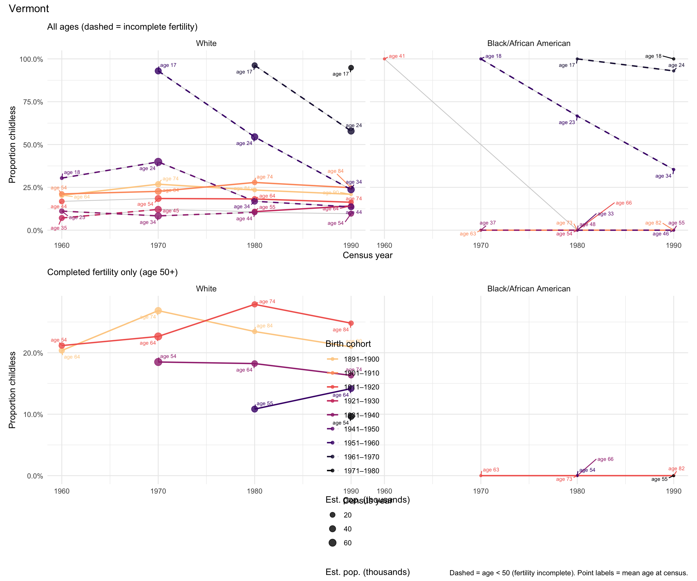
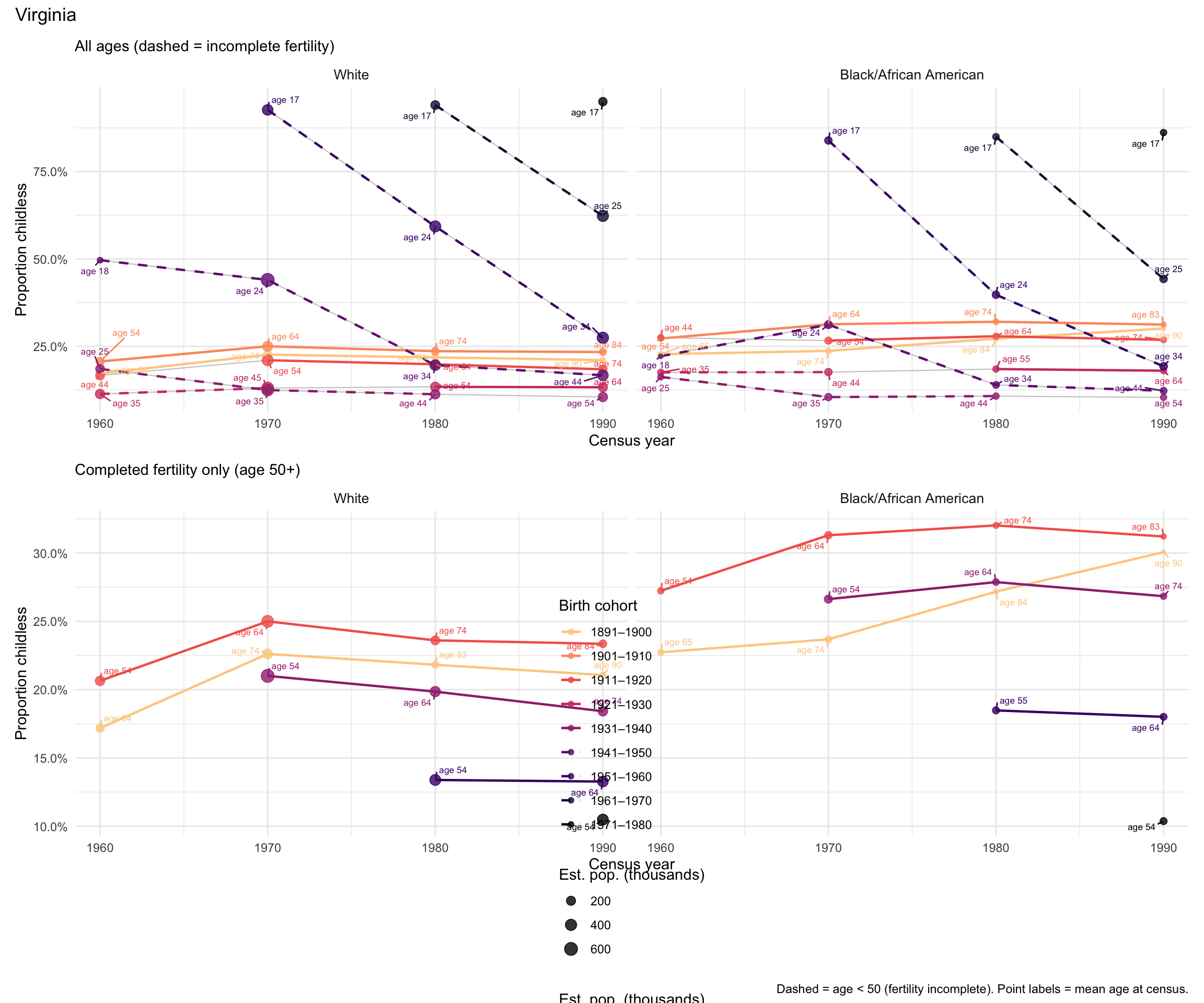
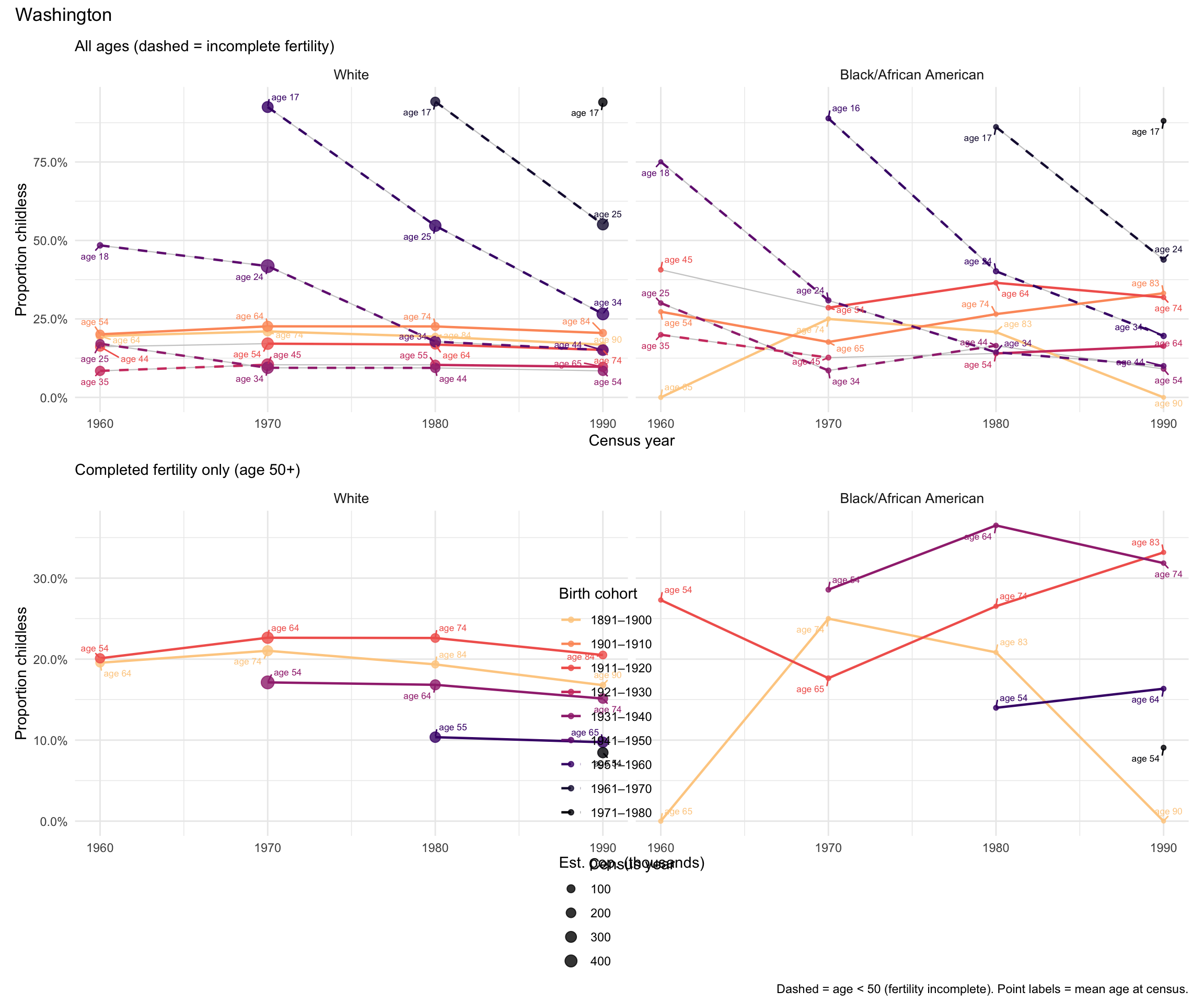
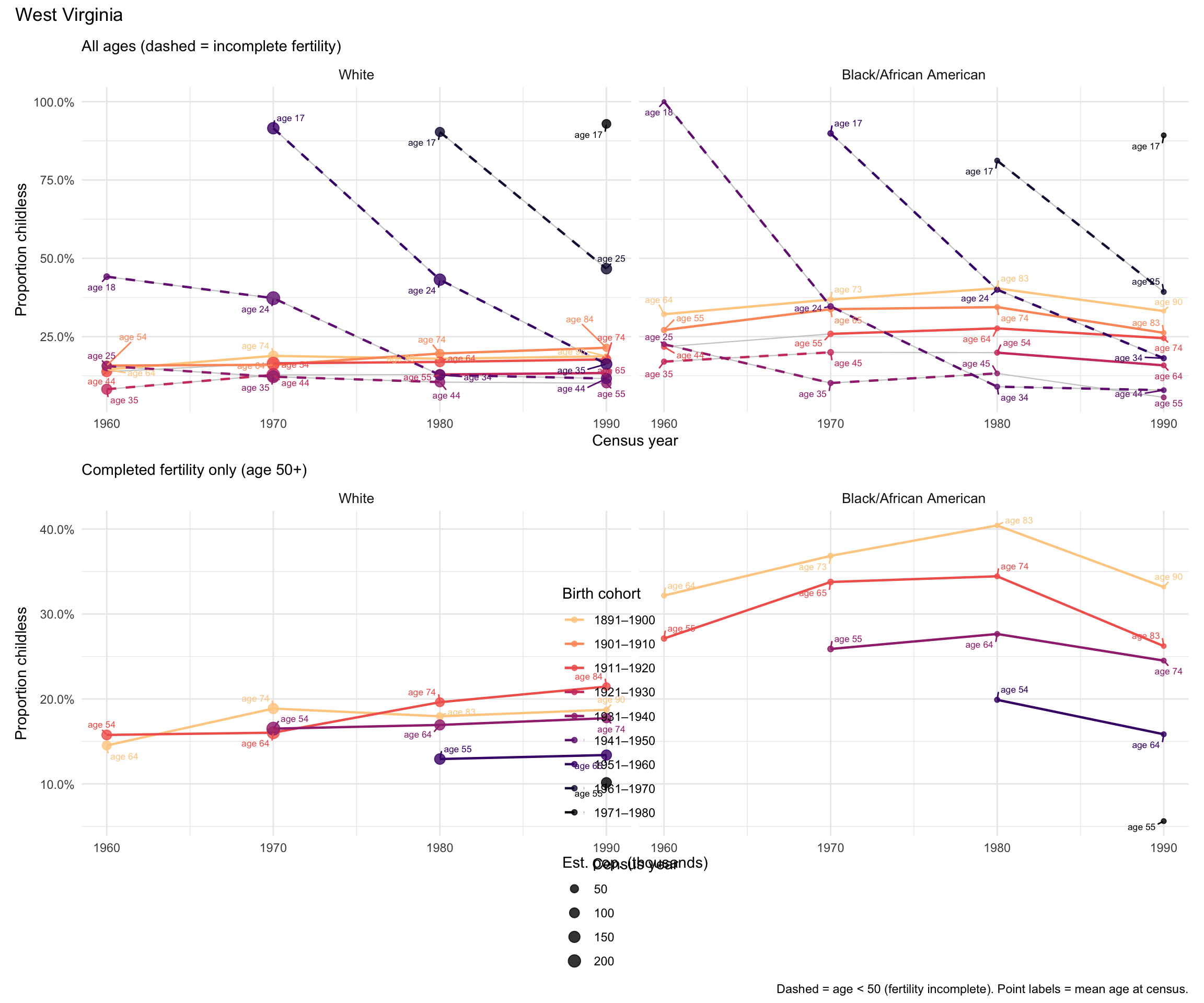
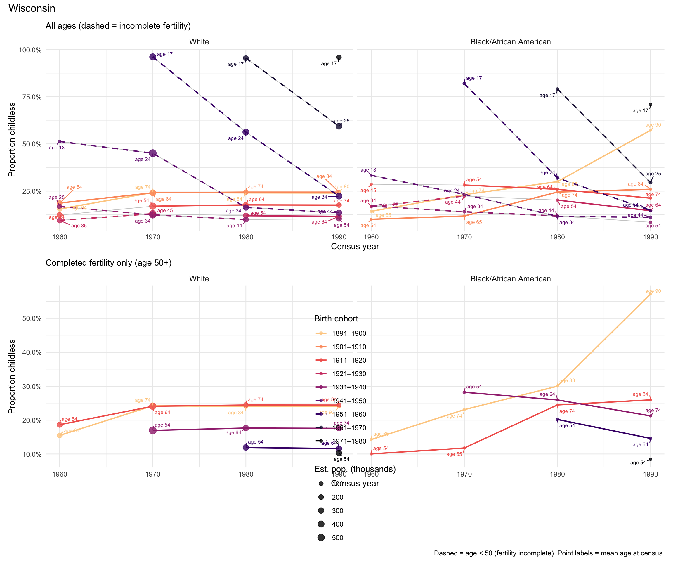
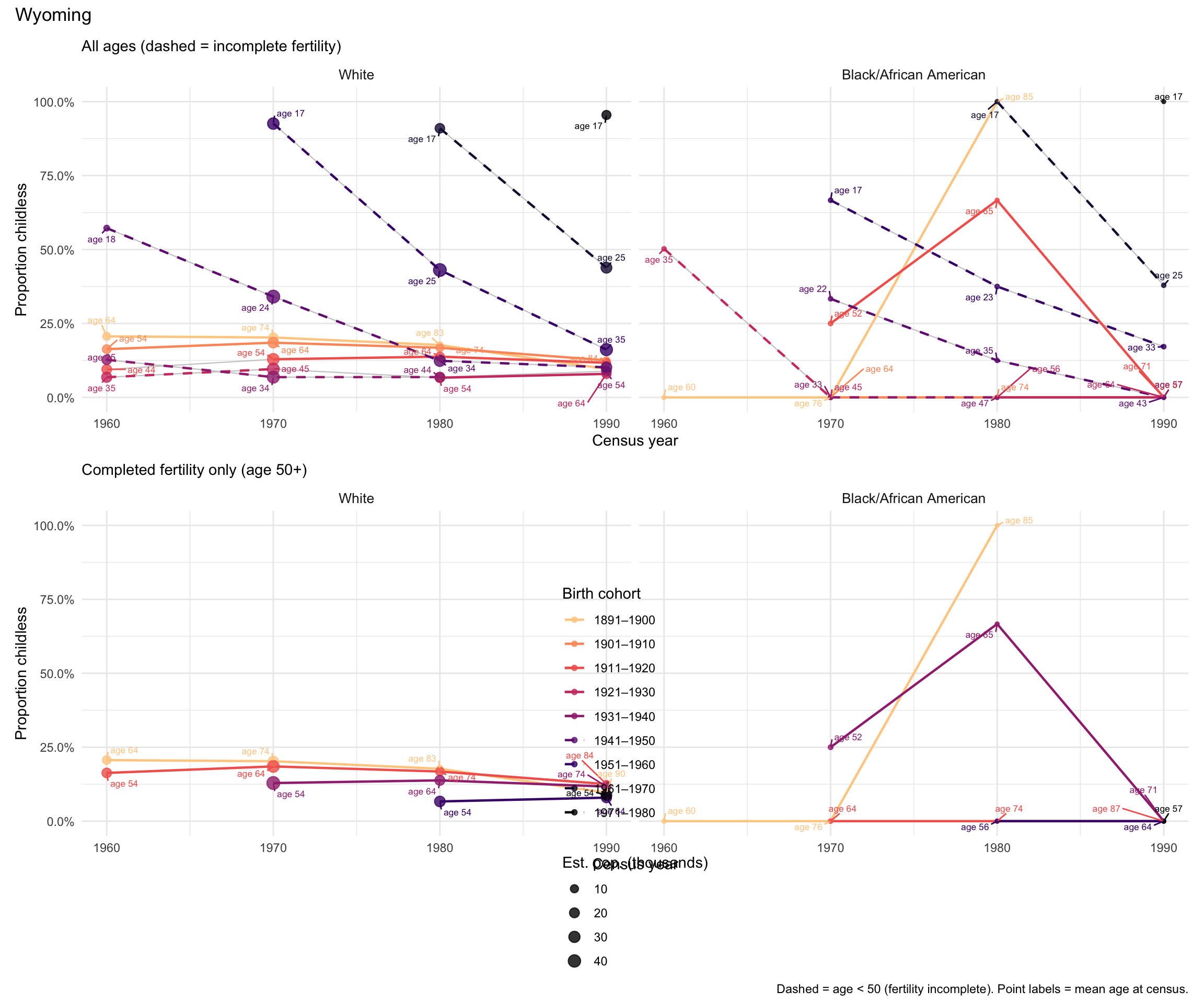
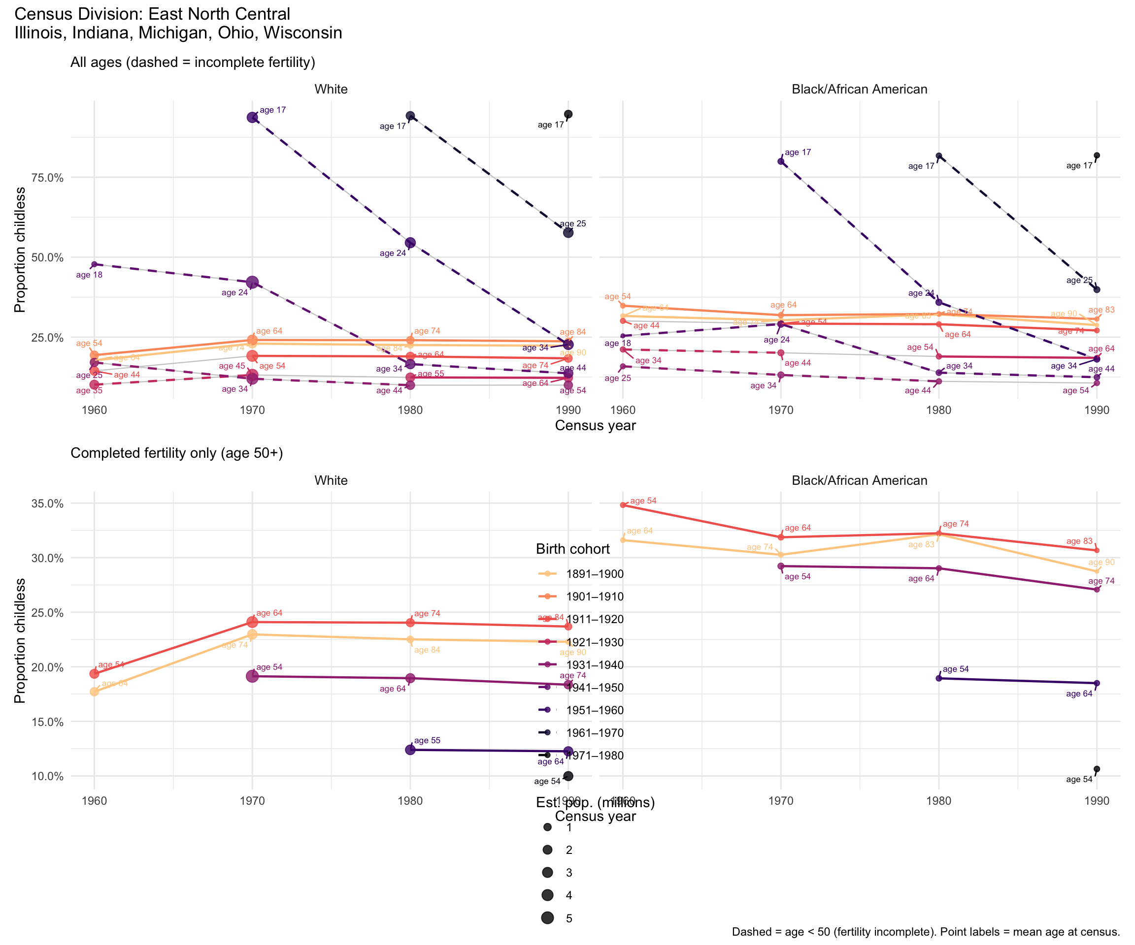
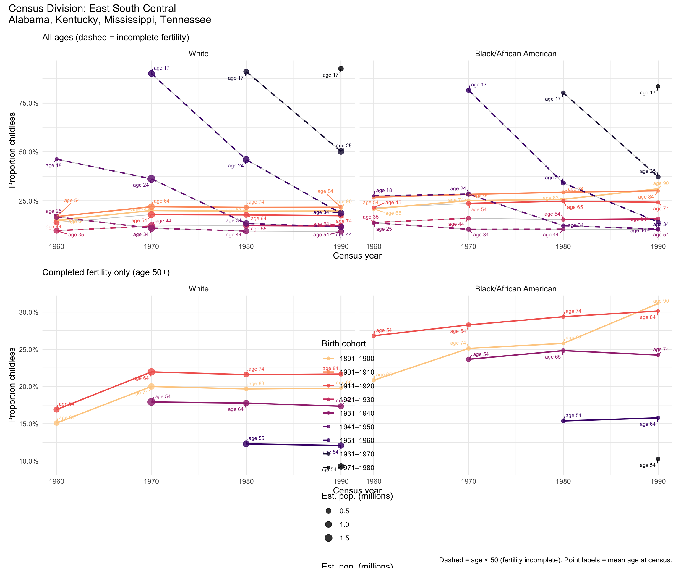
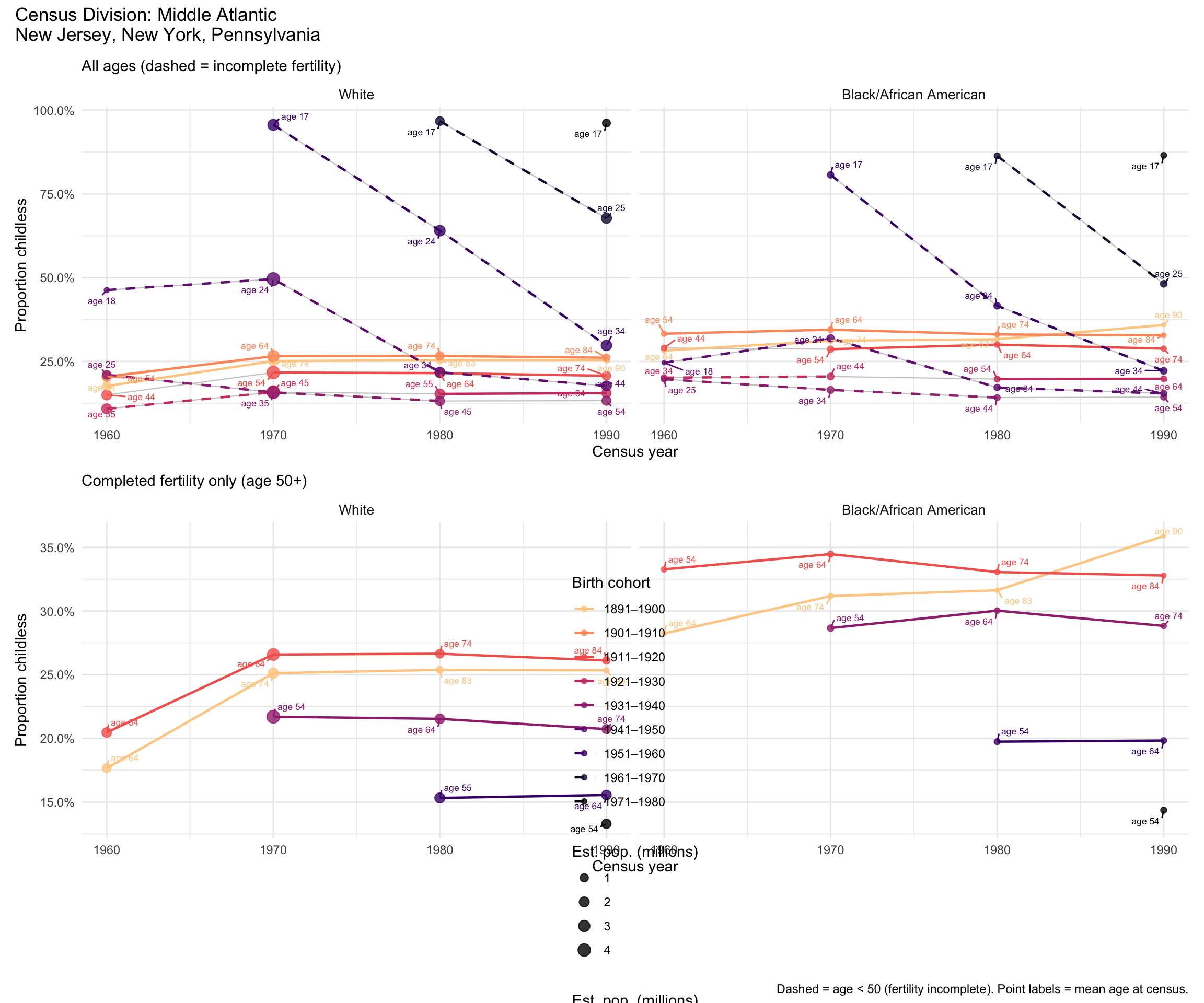
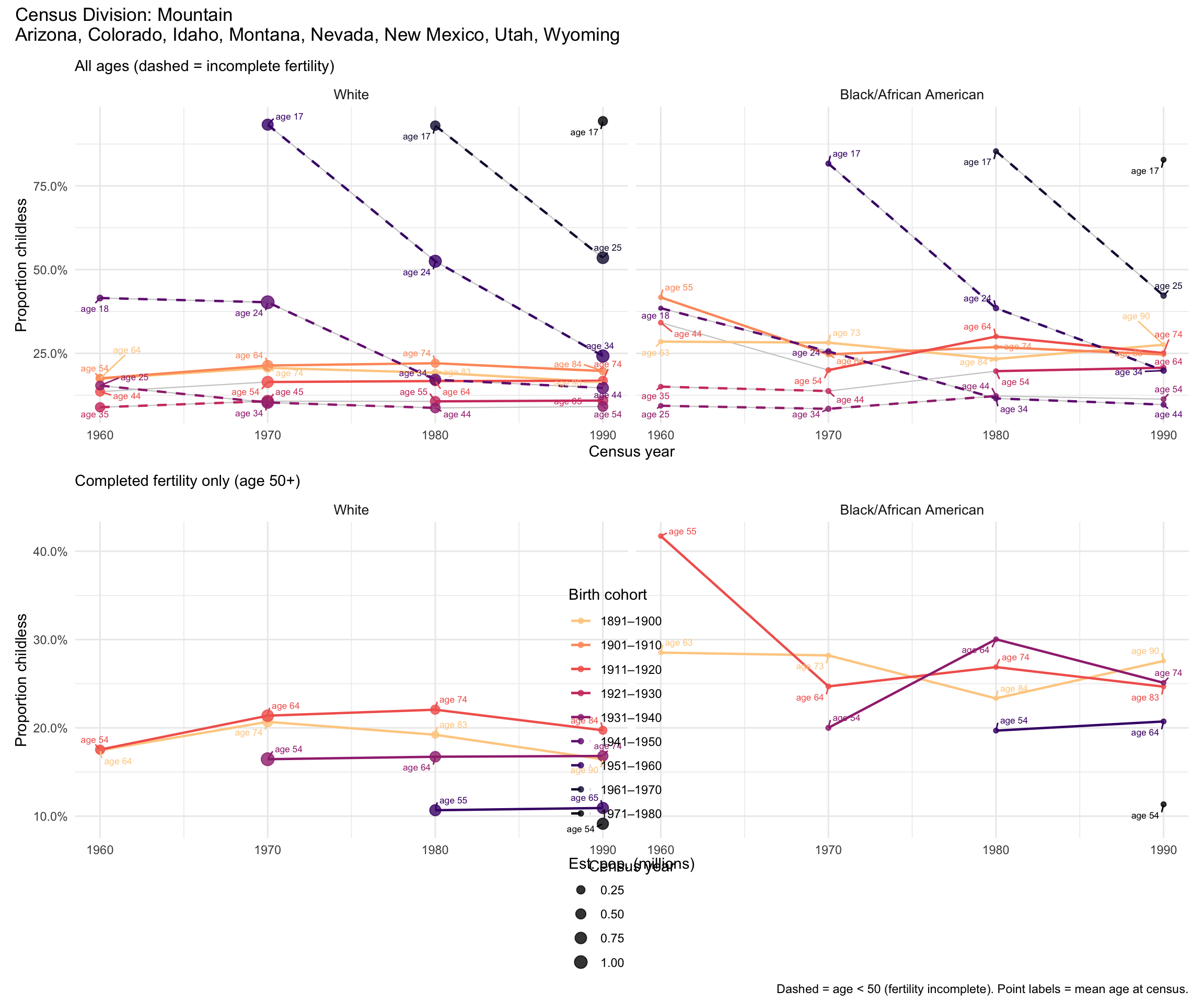
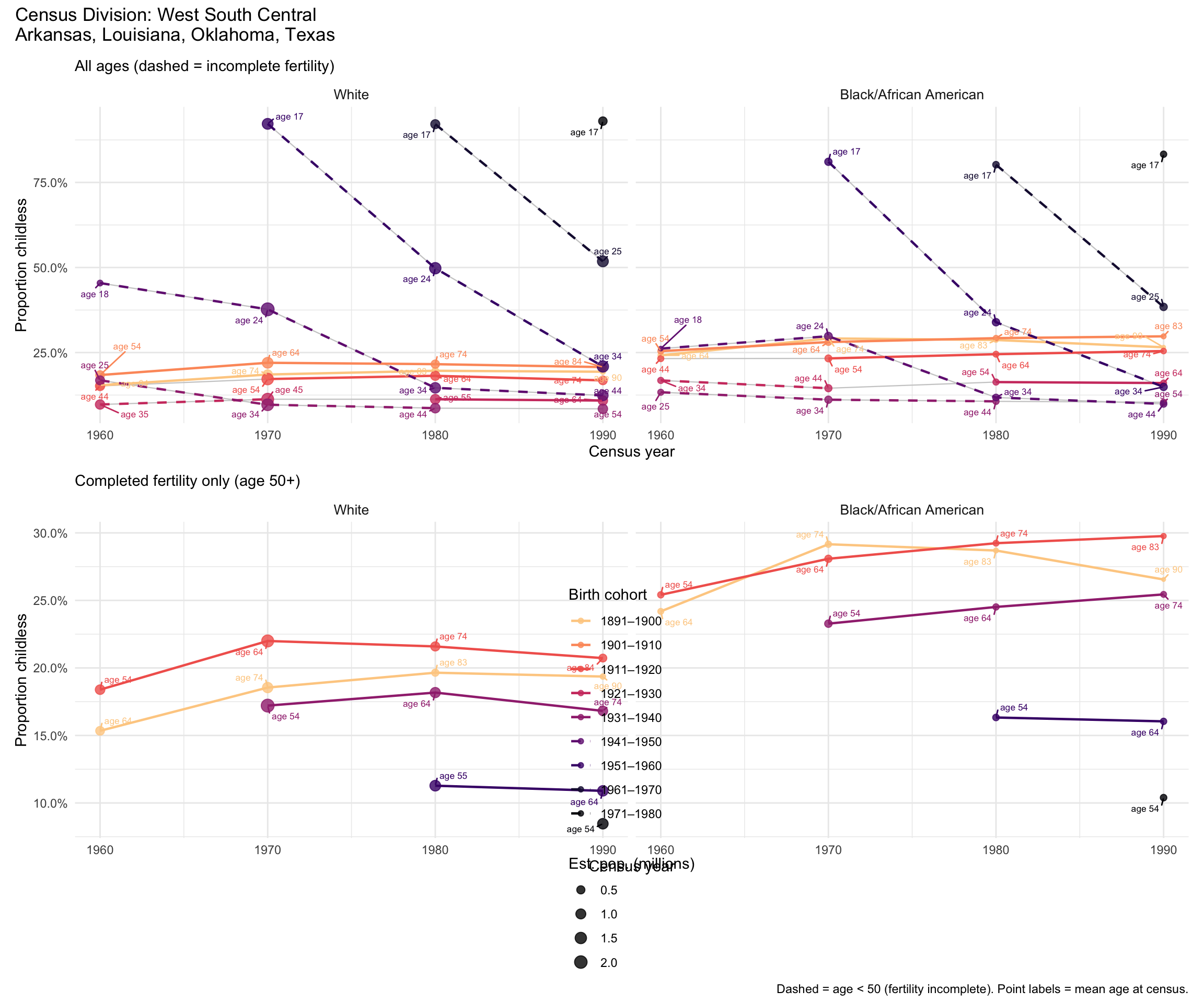
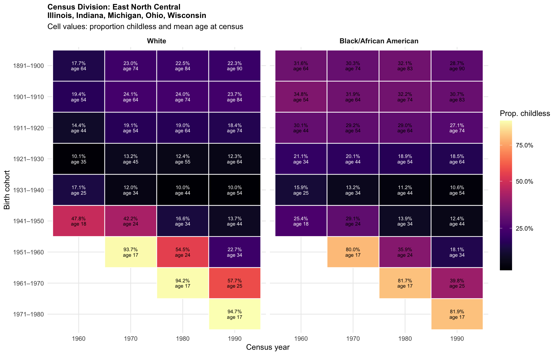
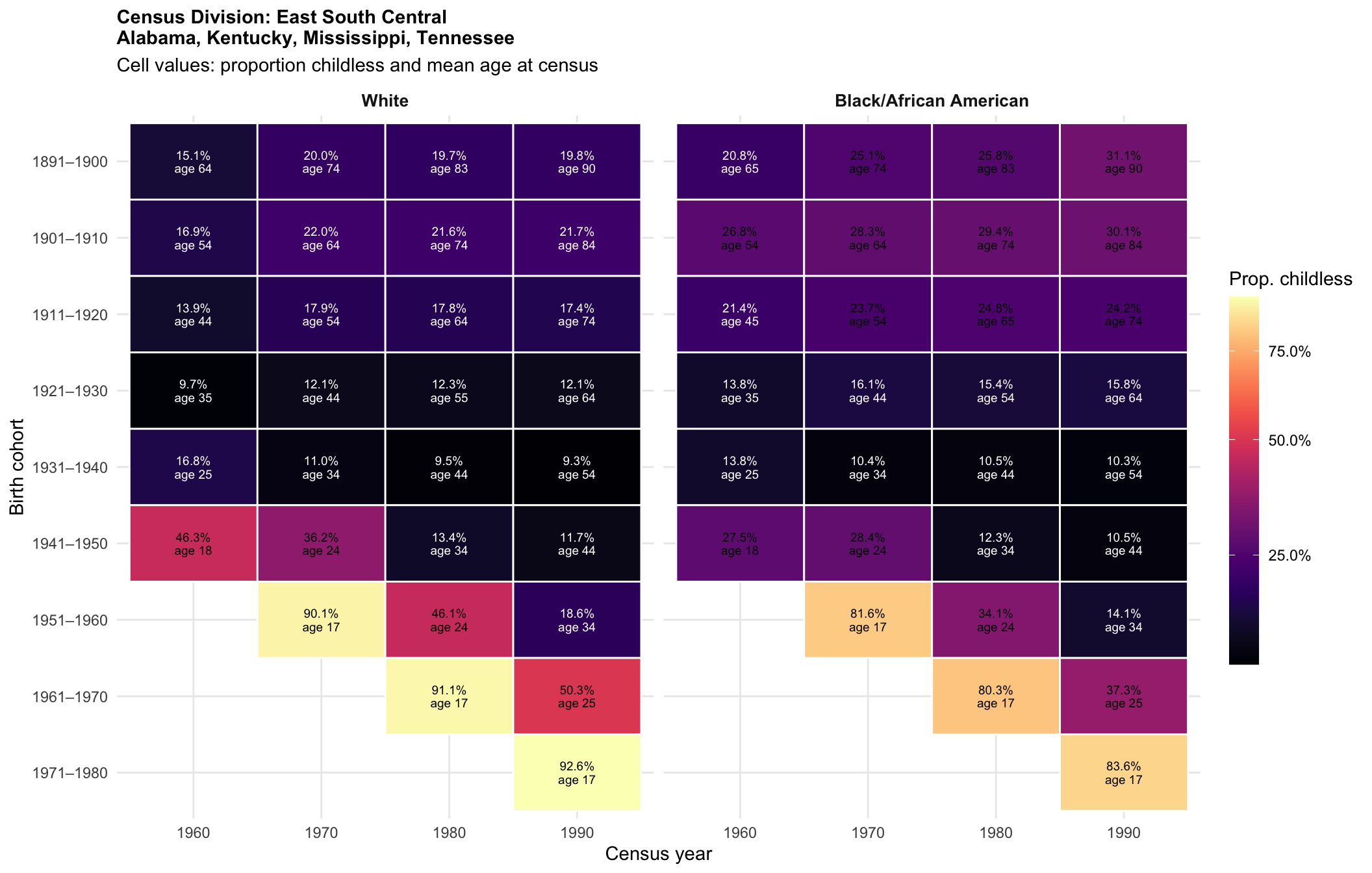
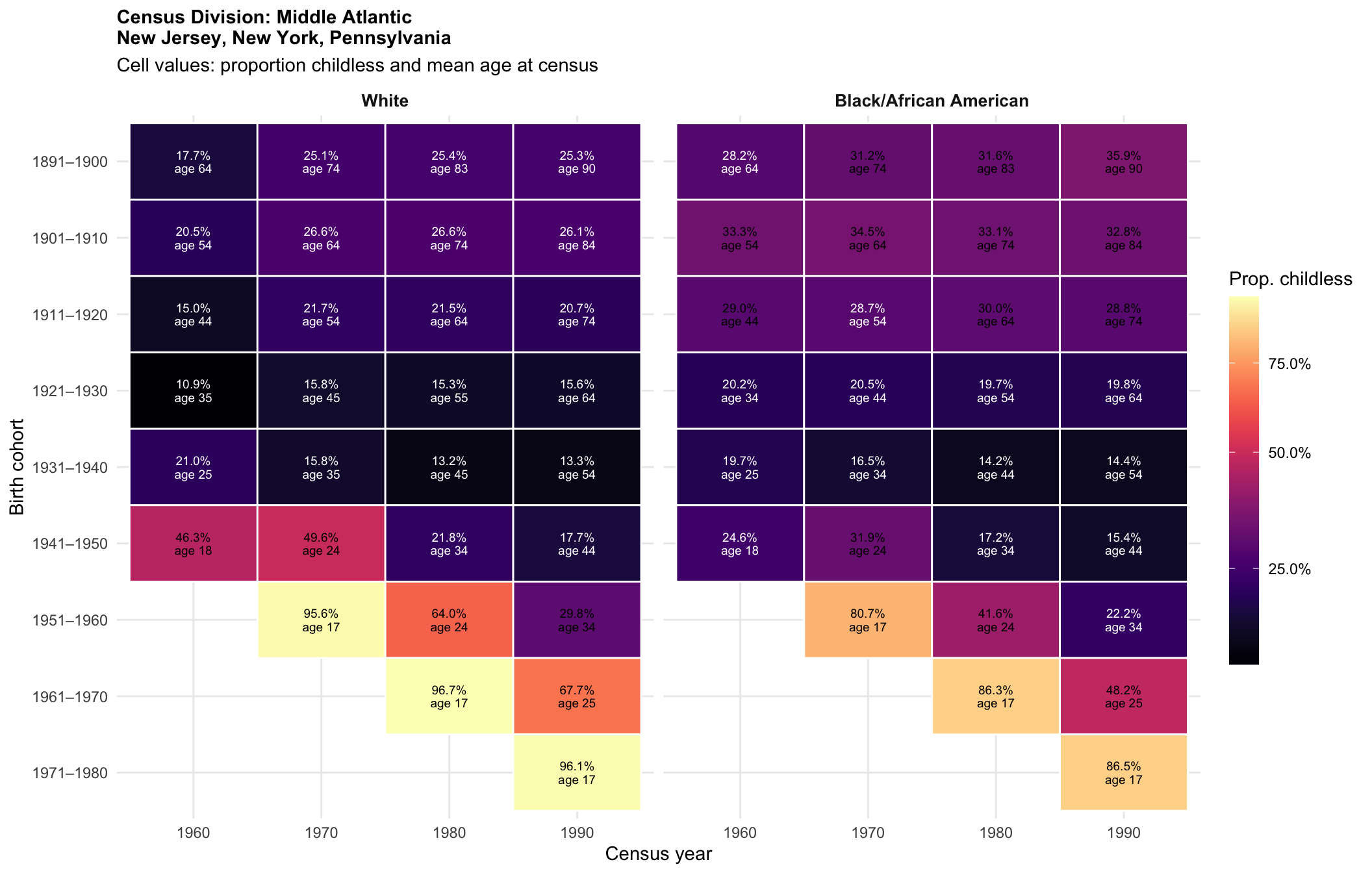
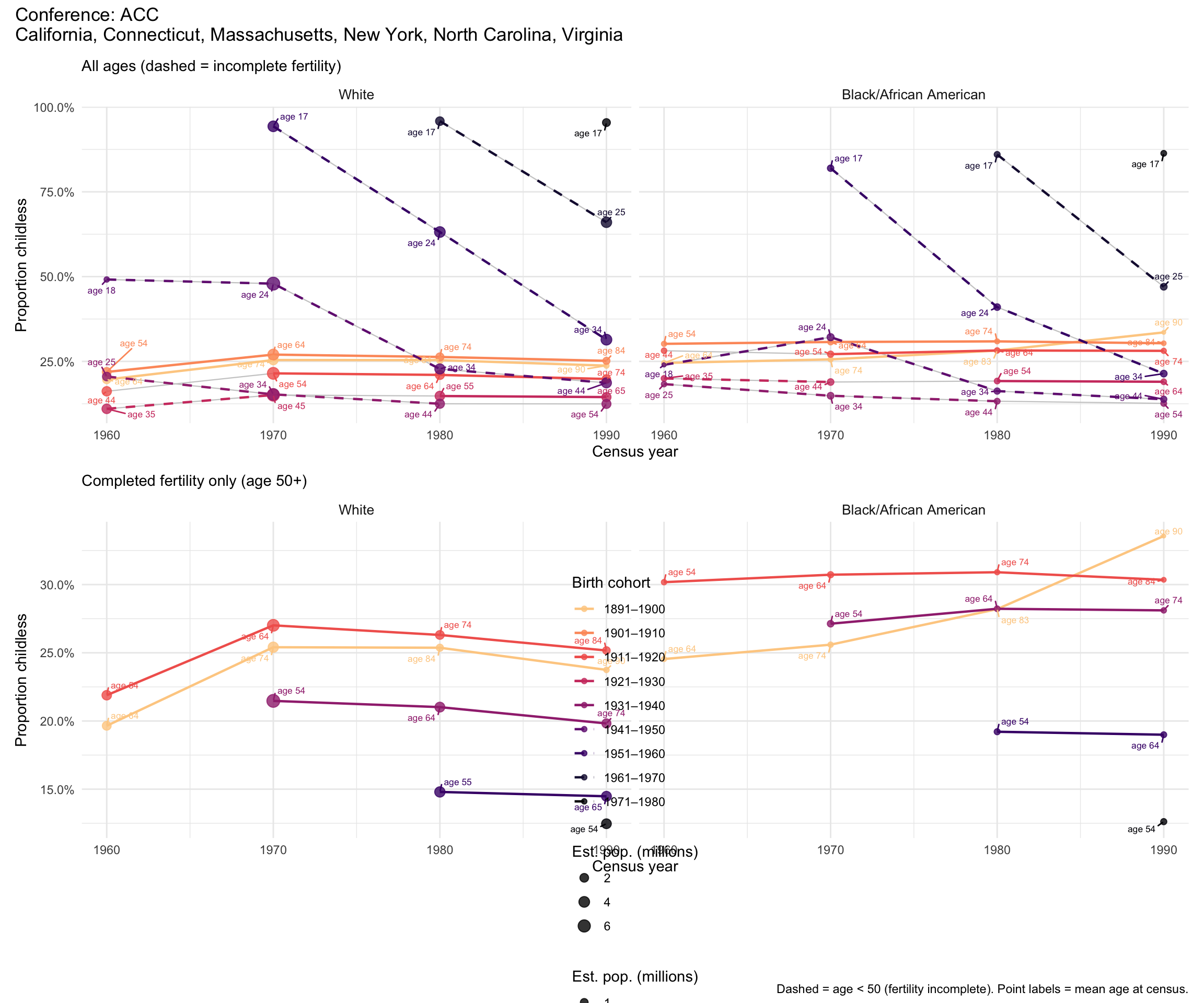
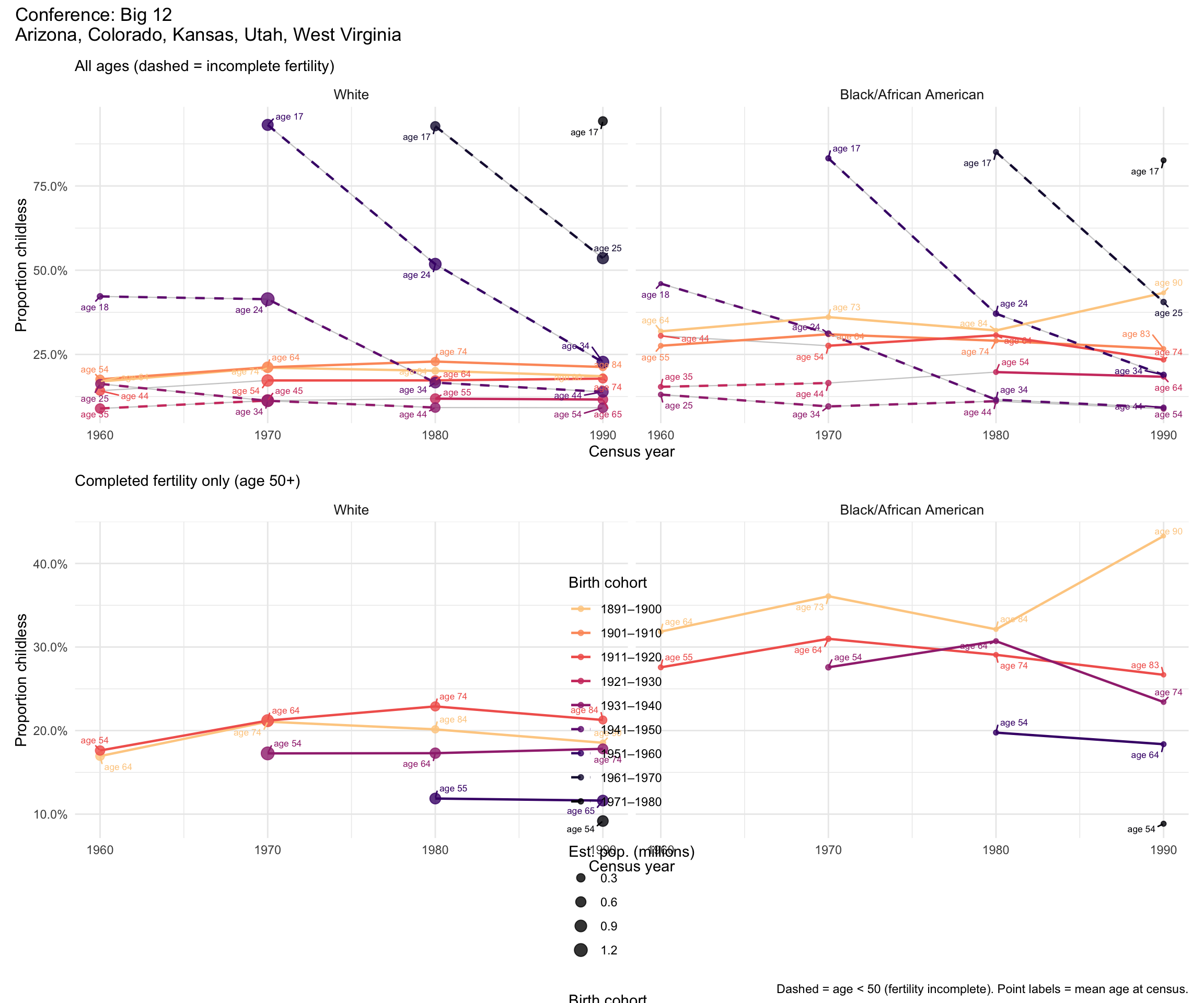
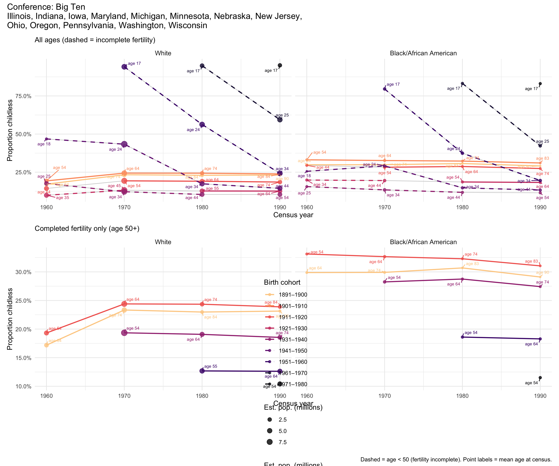
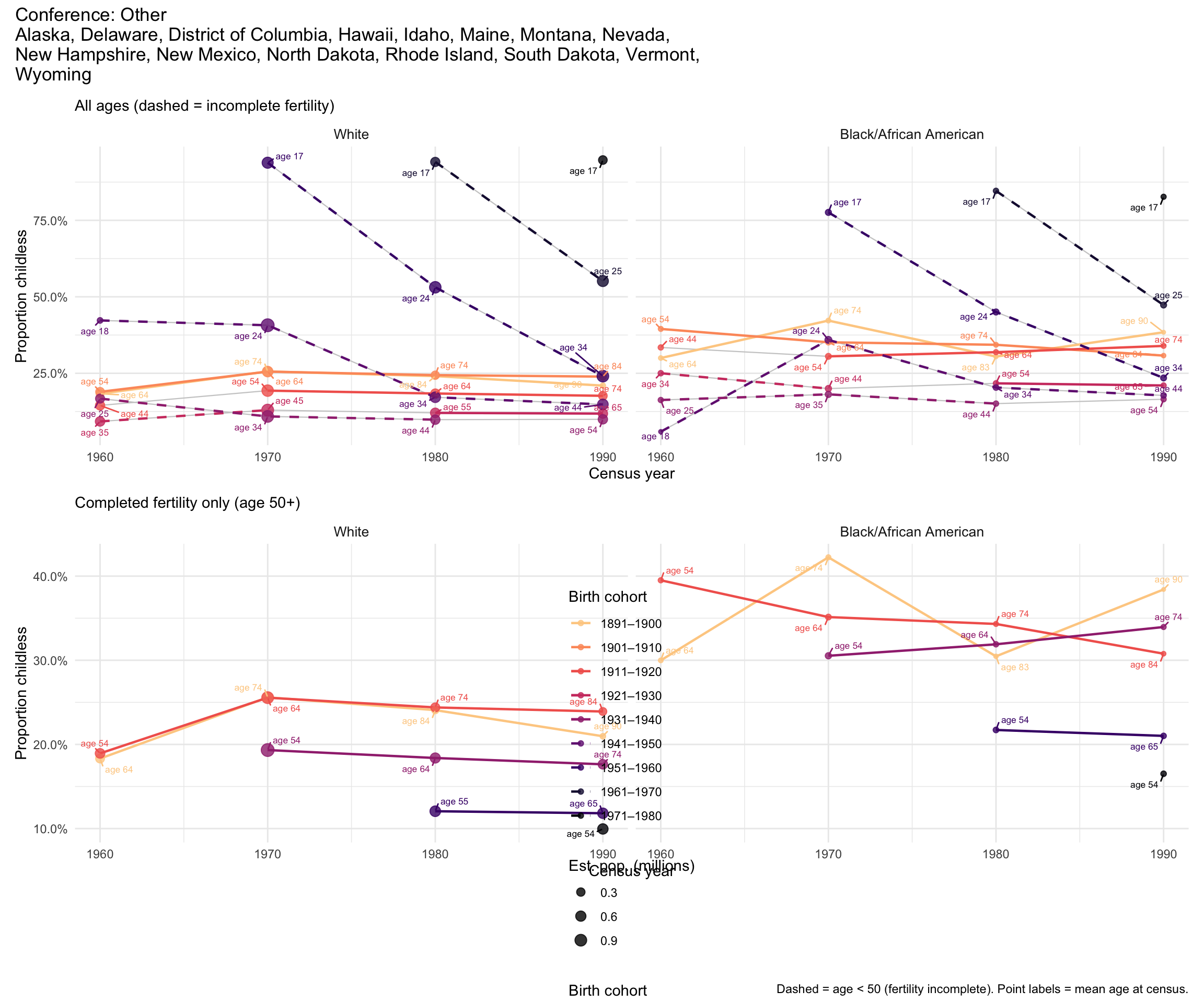
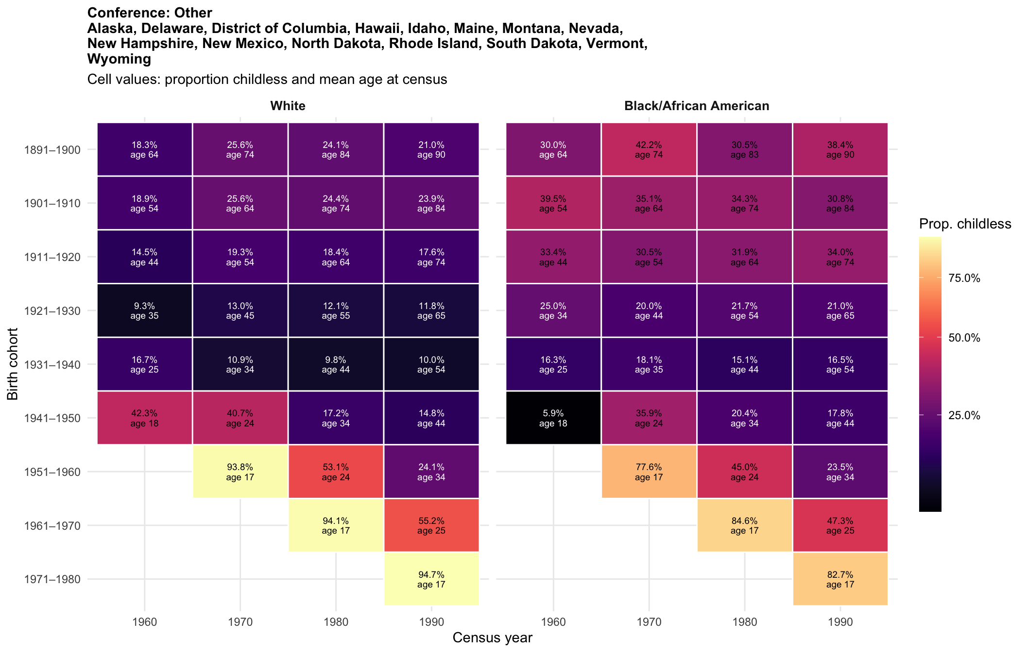
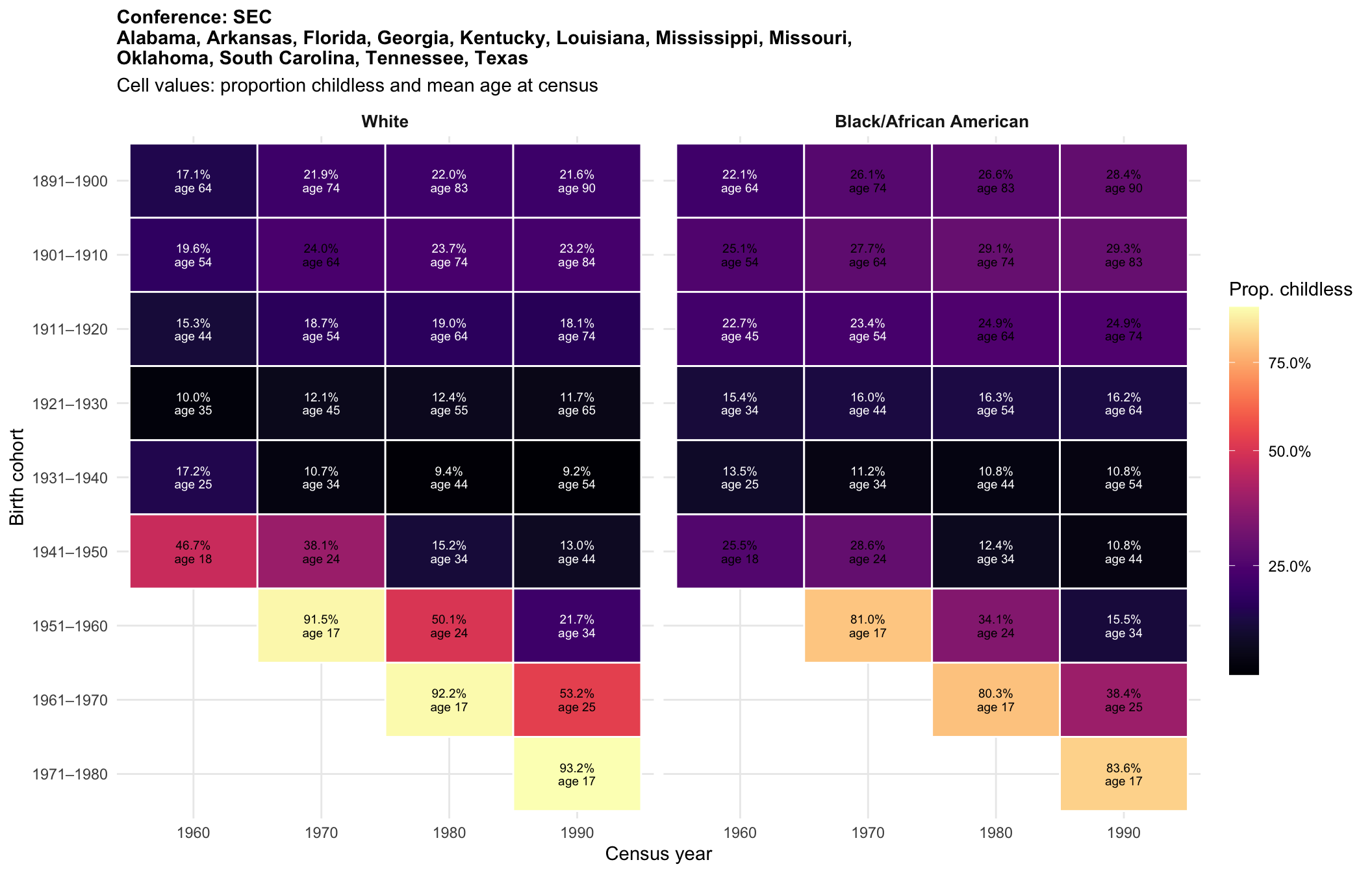
9. Cohort analysis: childlessness across age groups

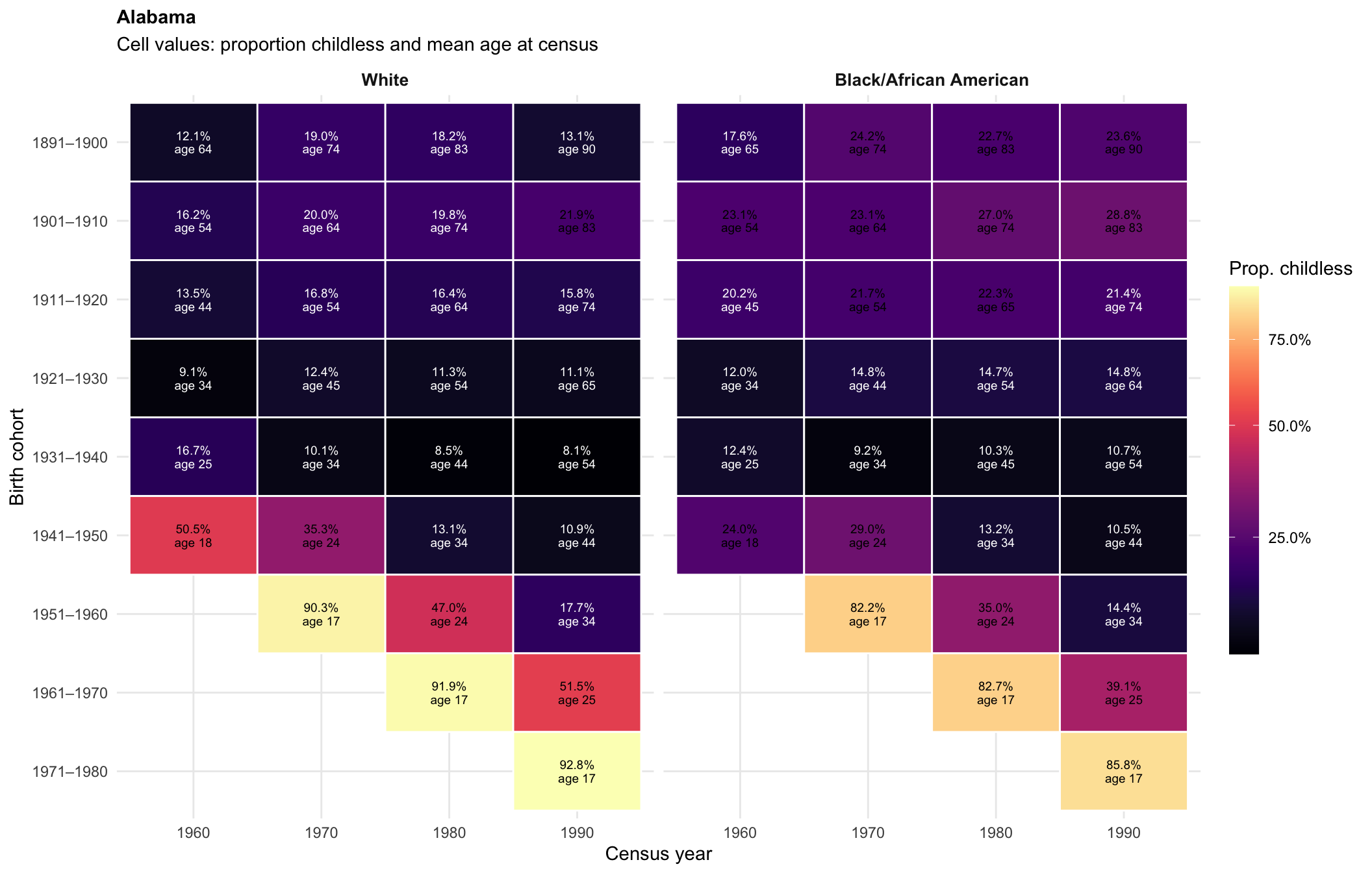
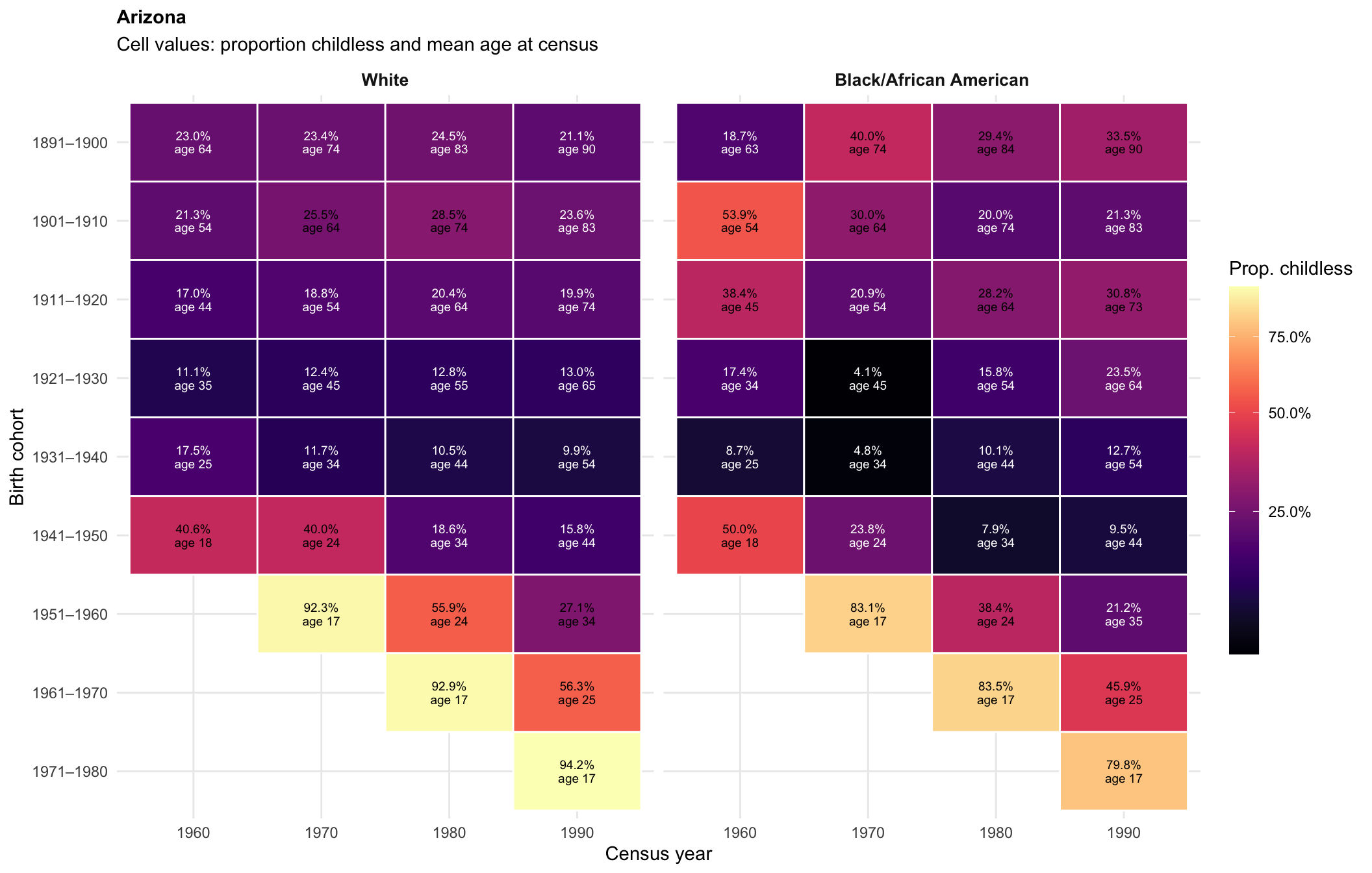
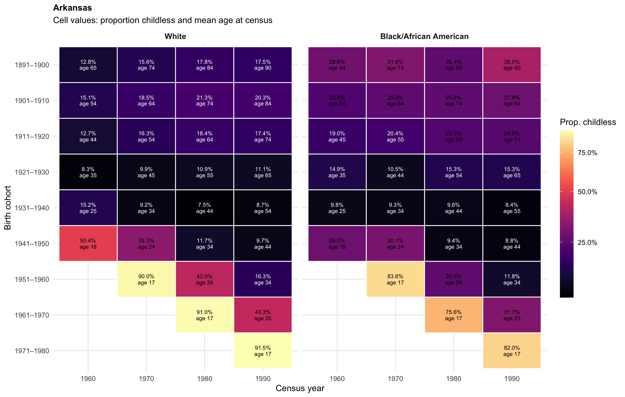
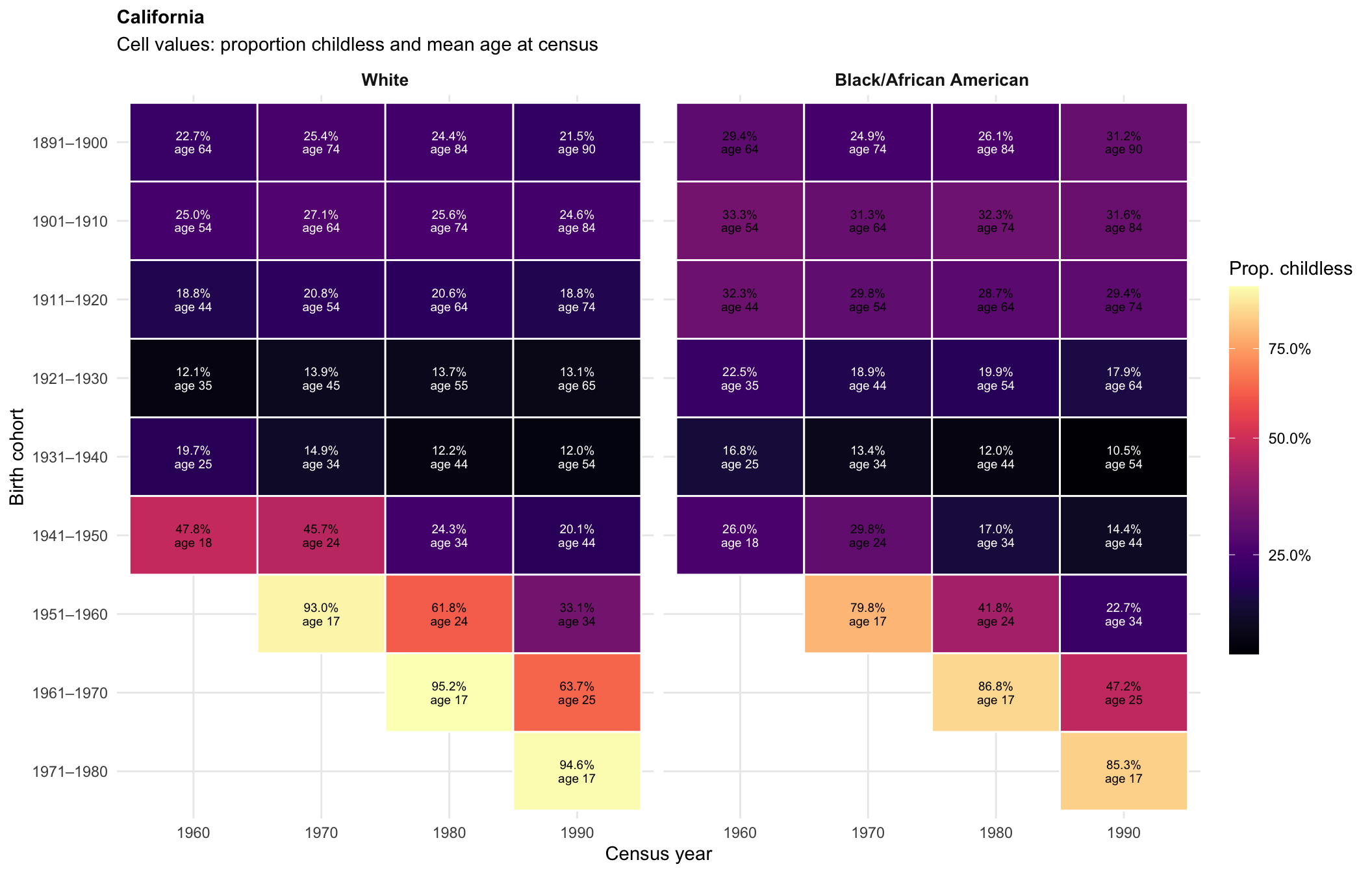
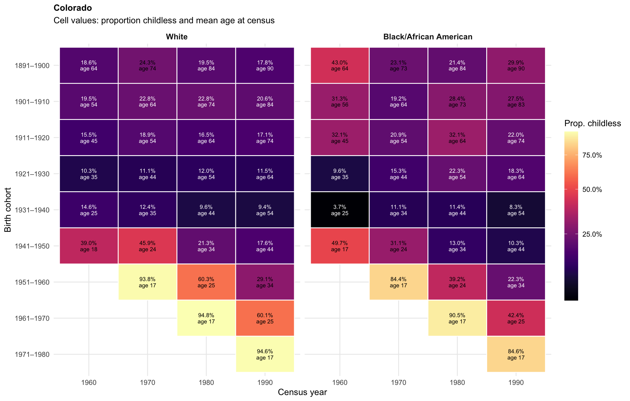
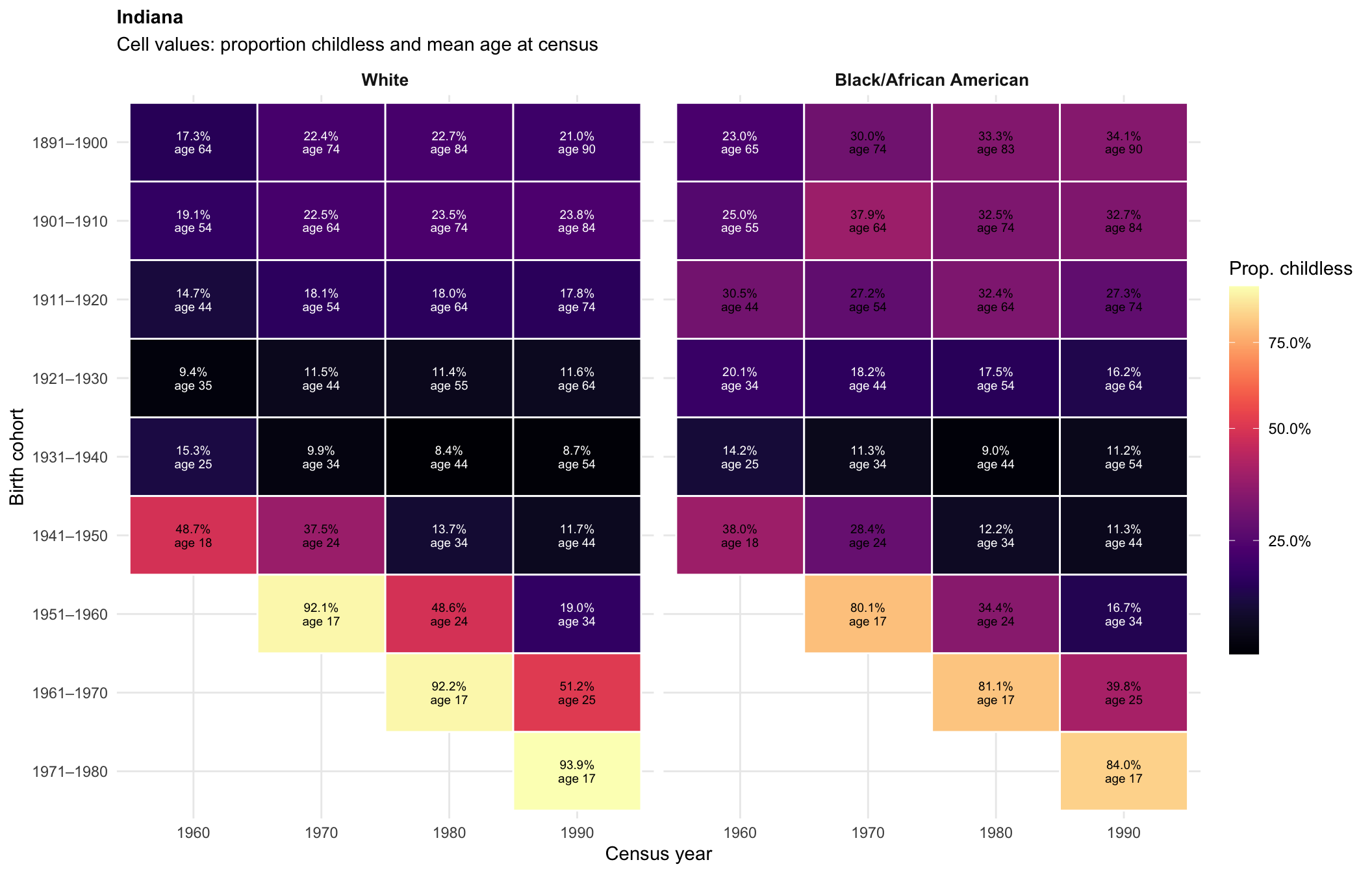
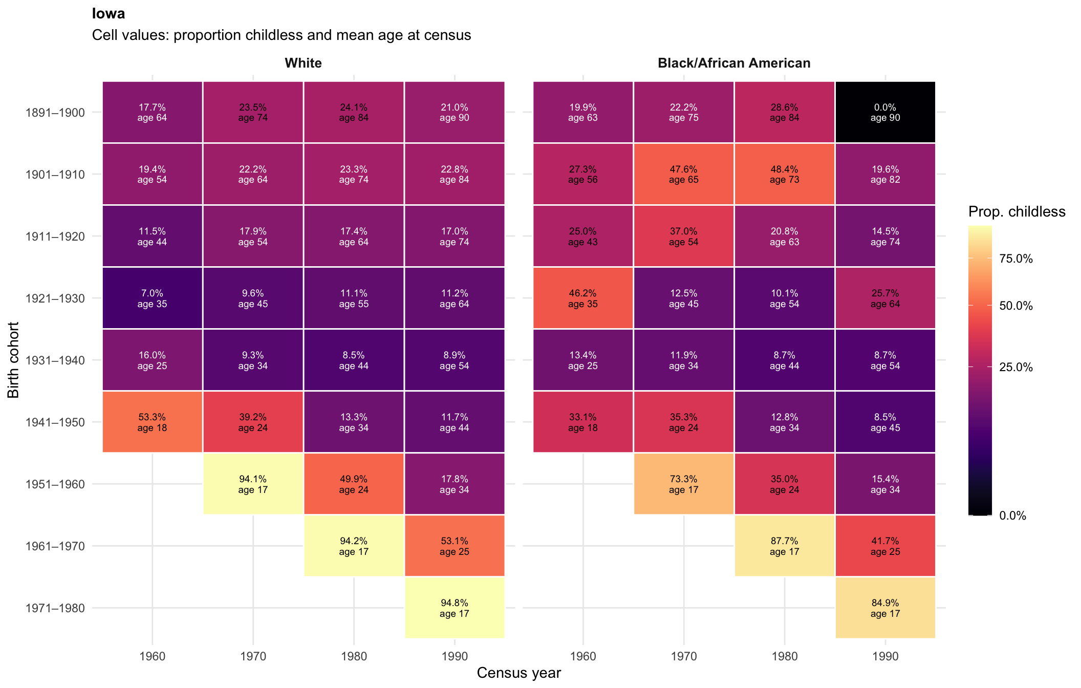
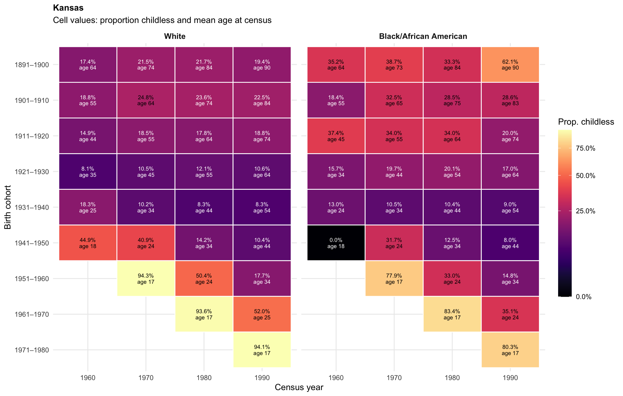
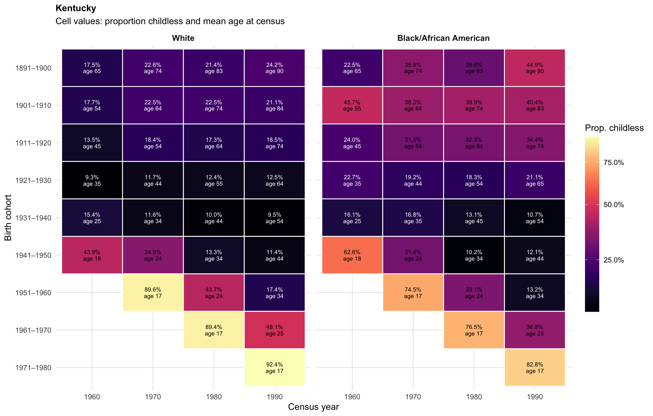
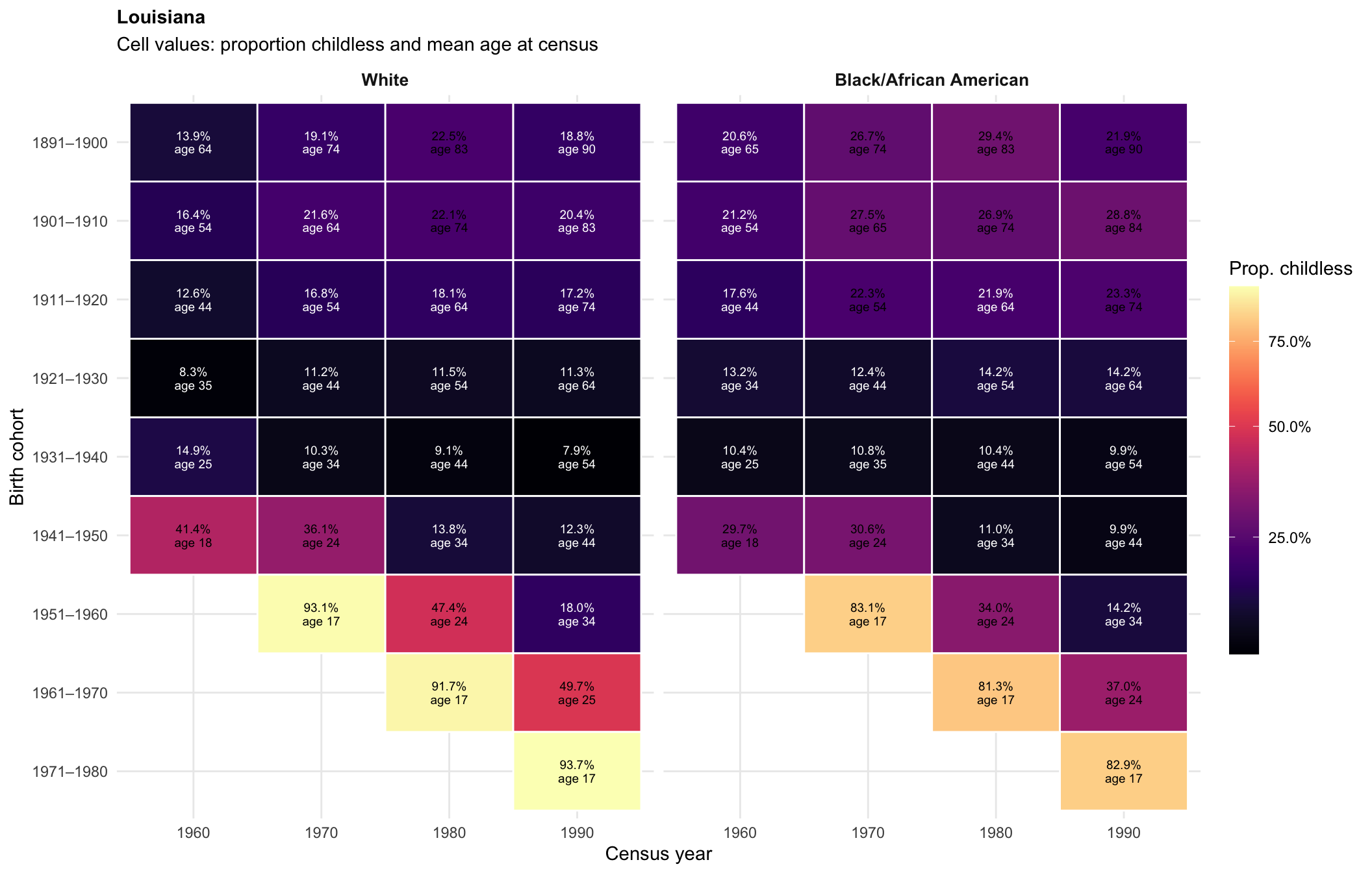
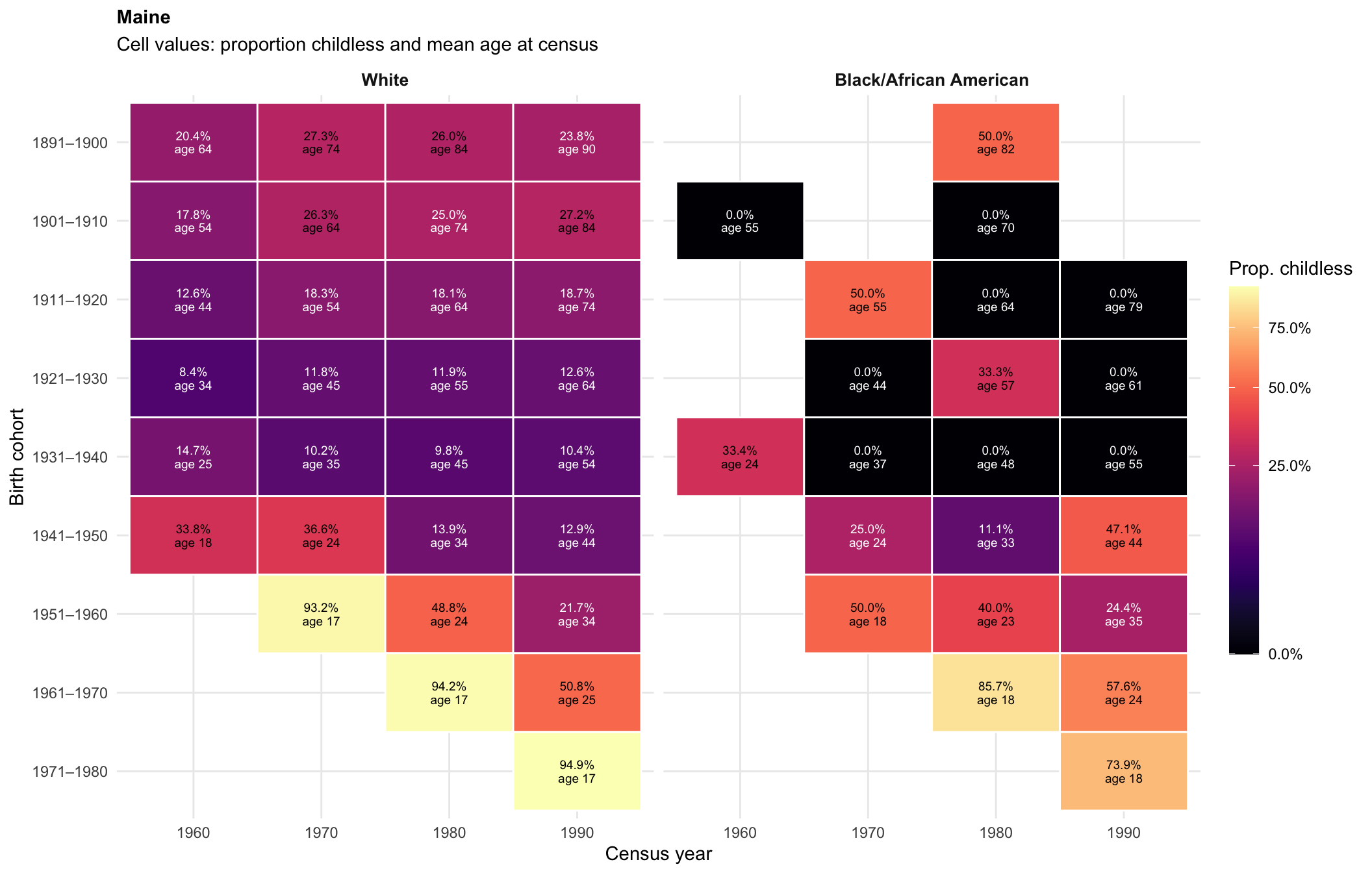
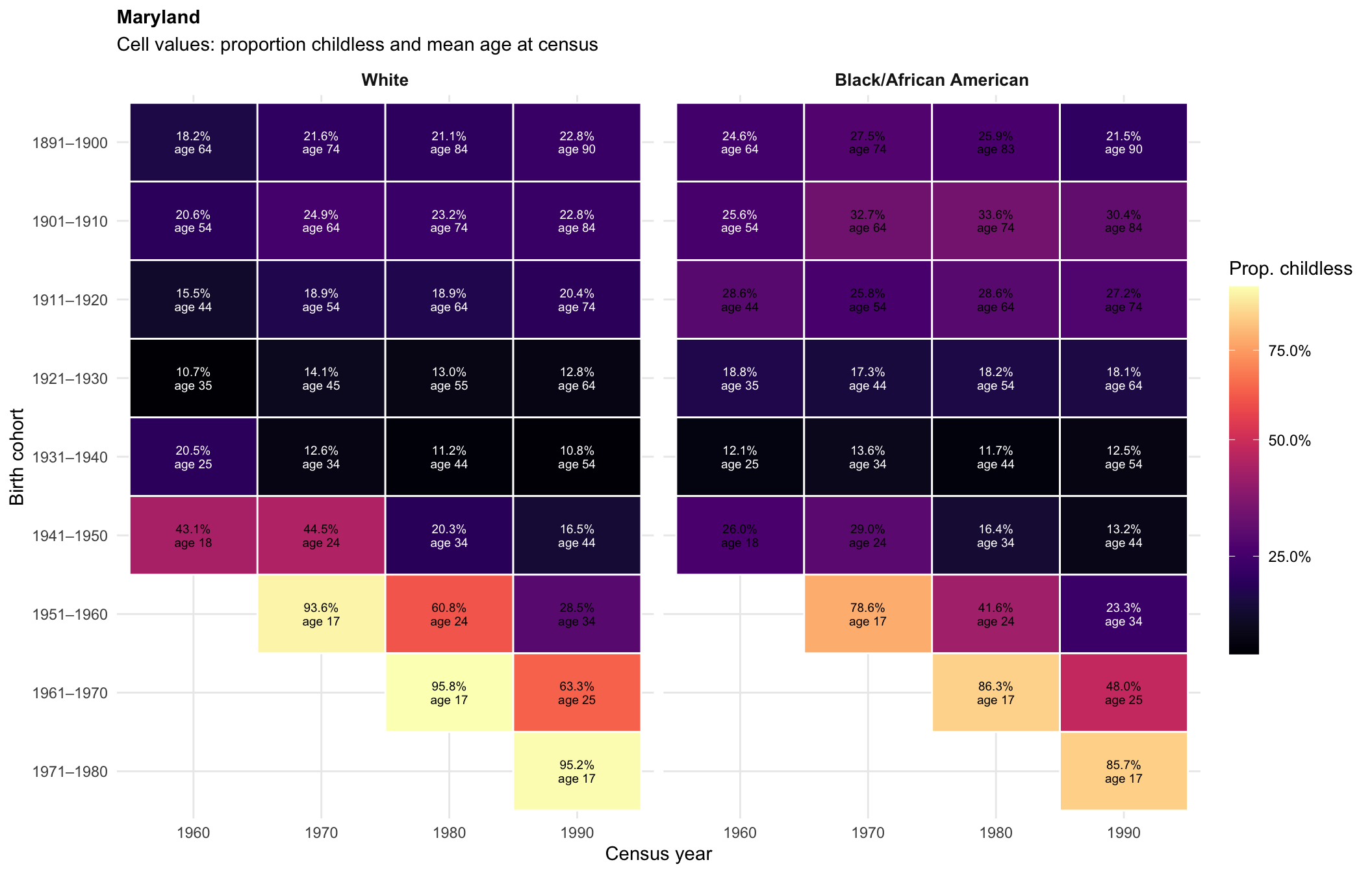
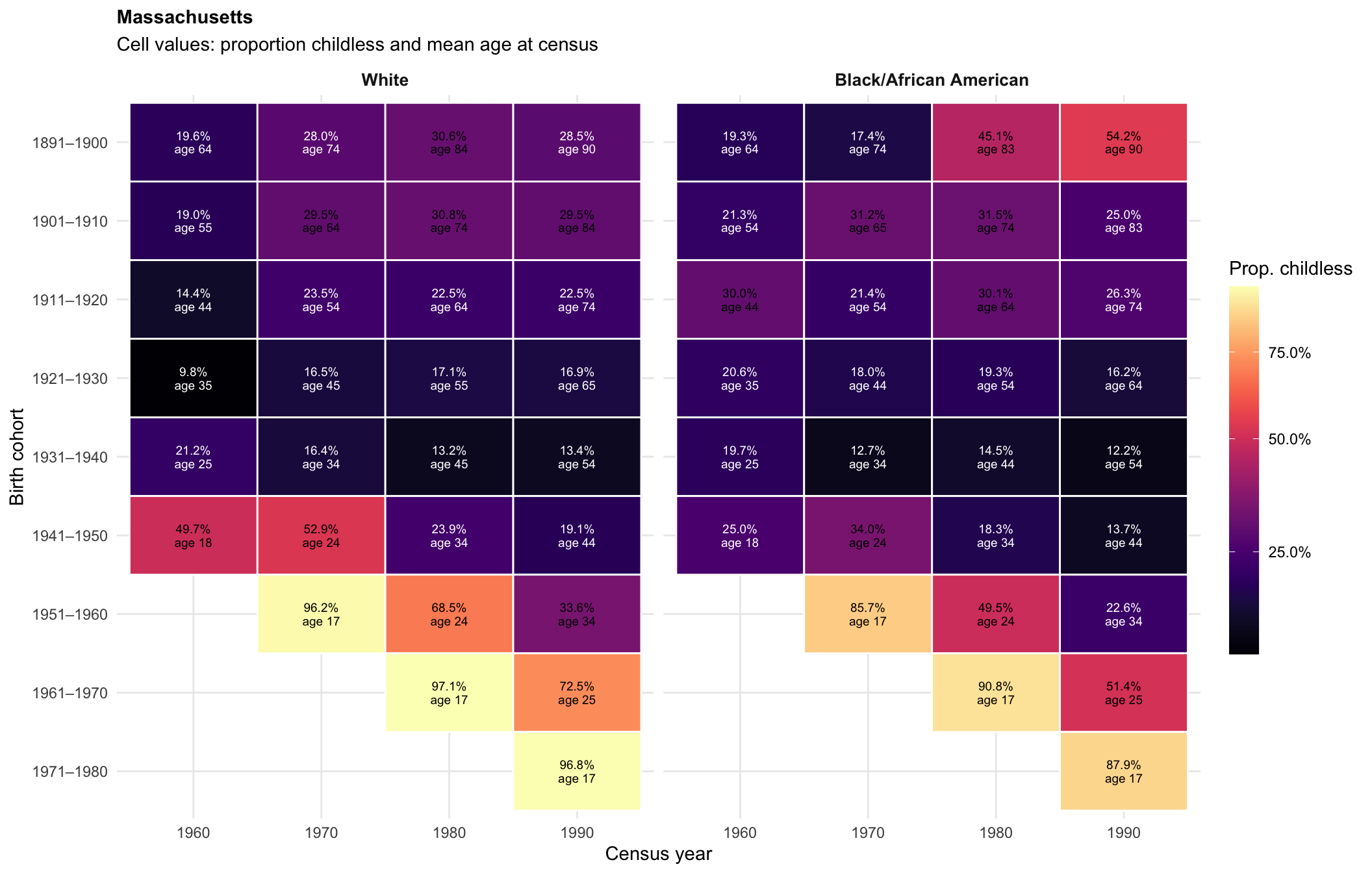
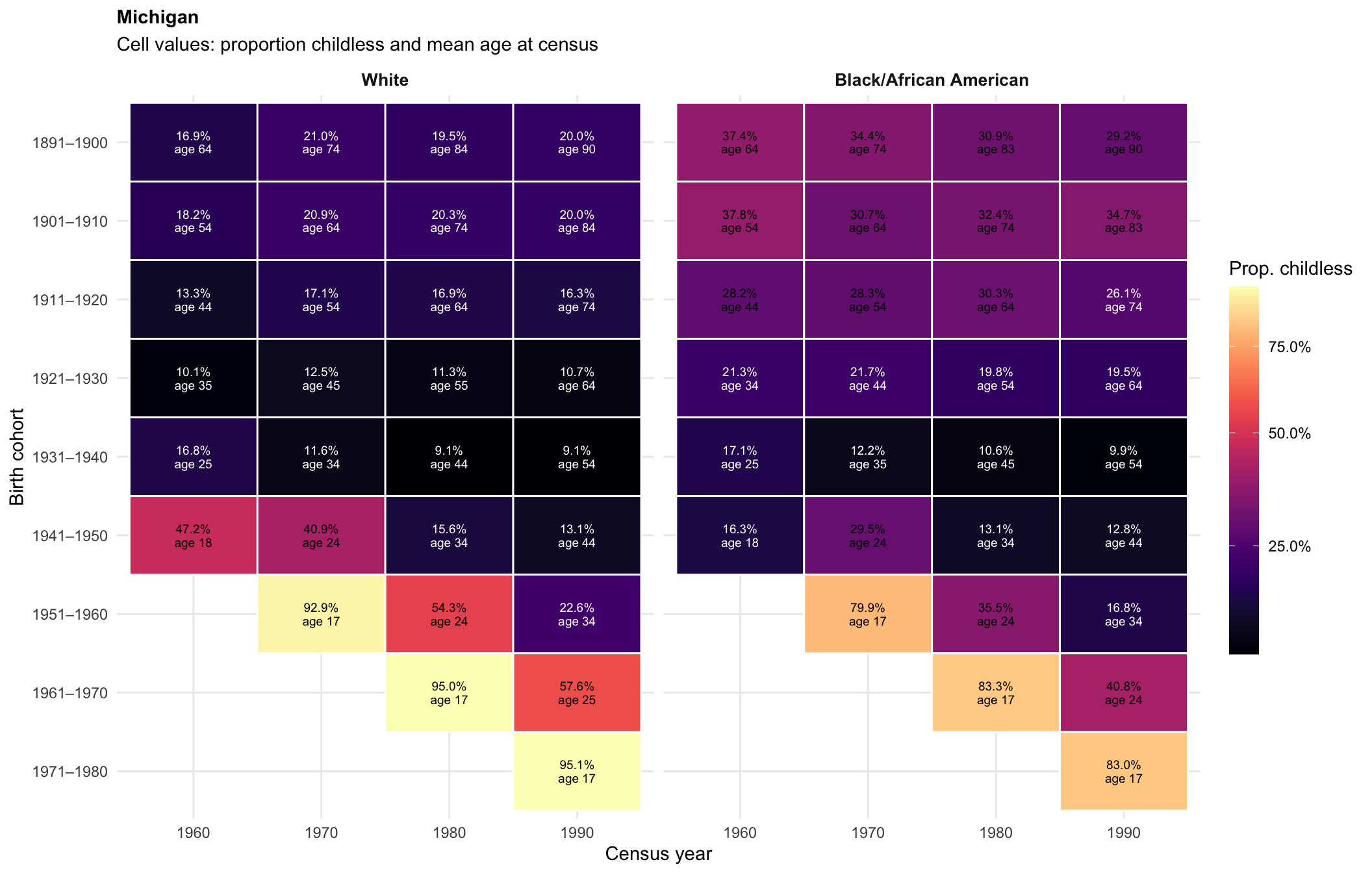
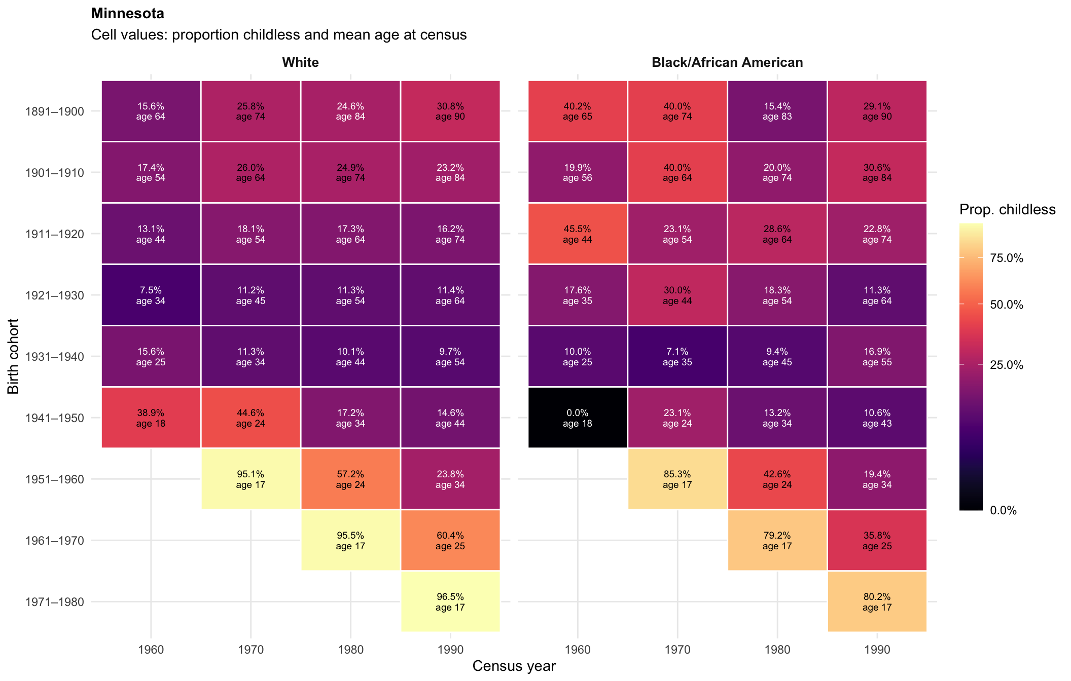
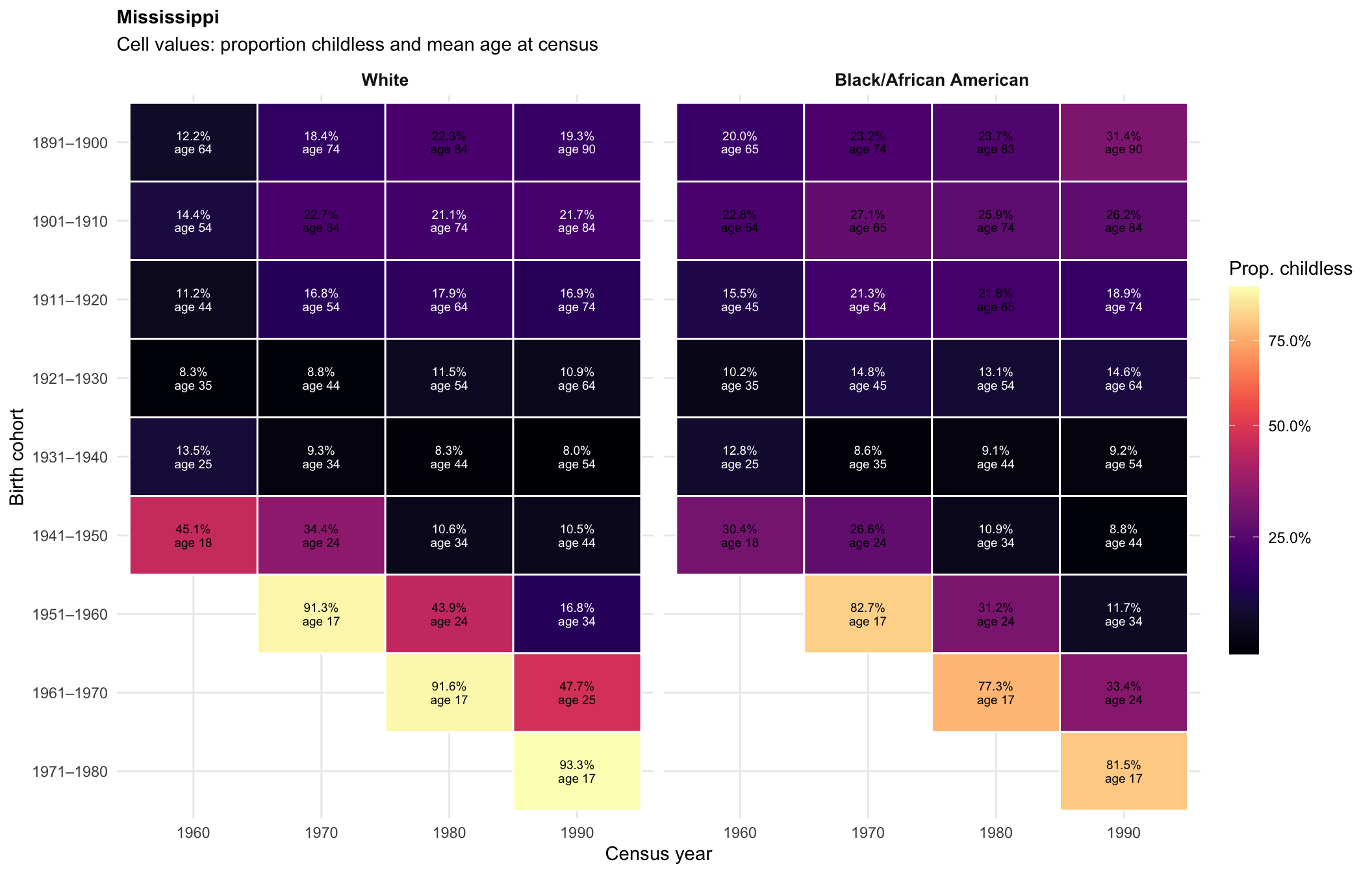
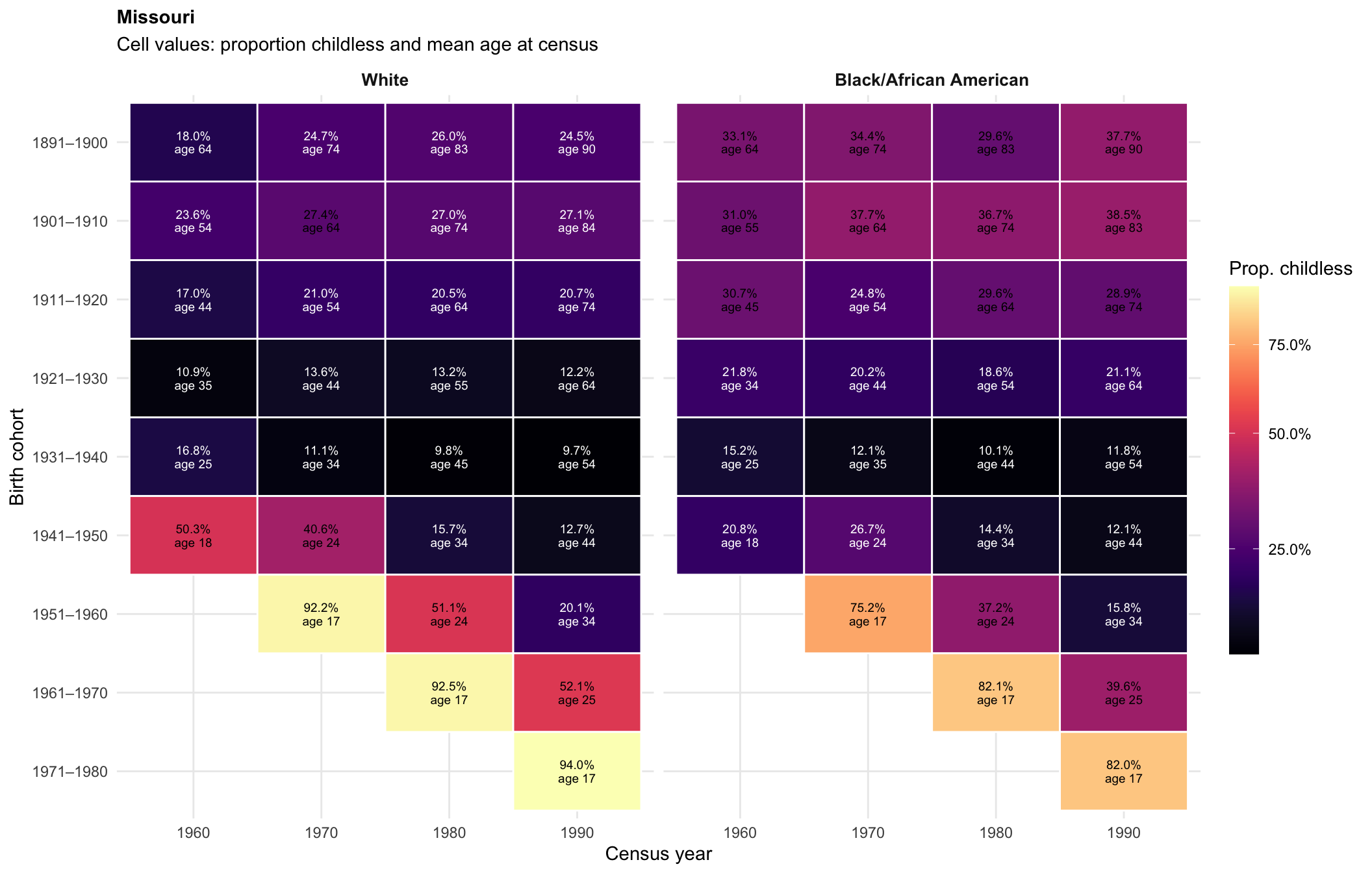
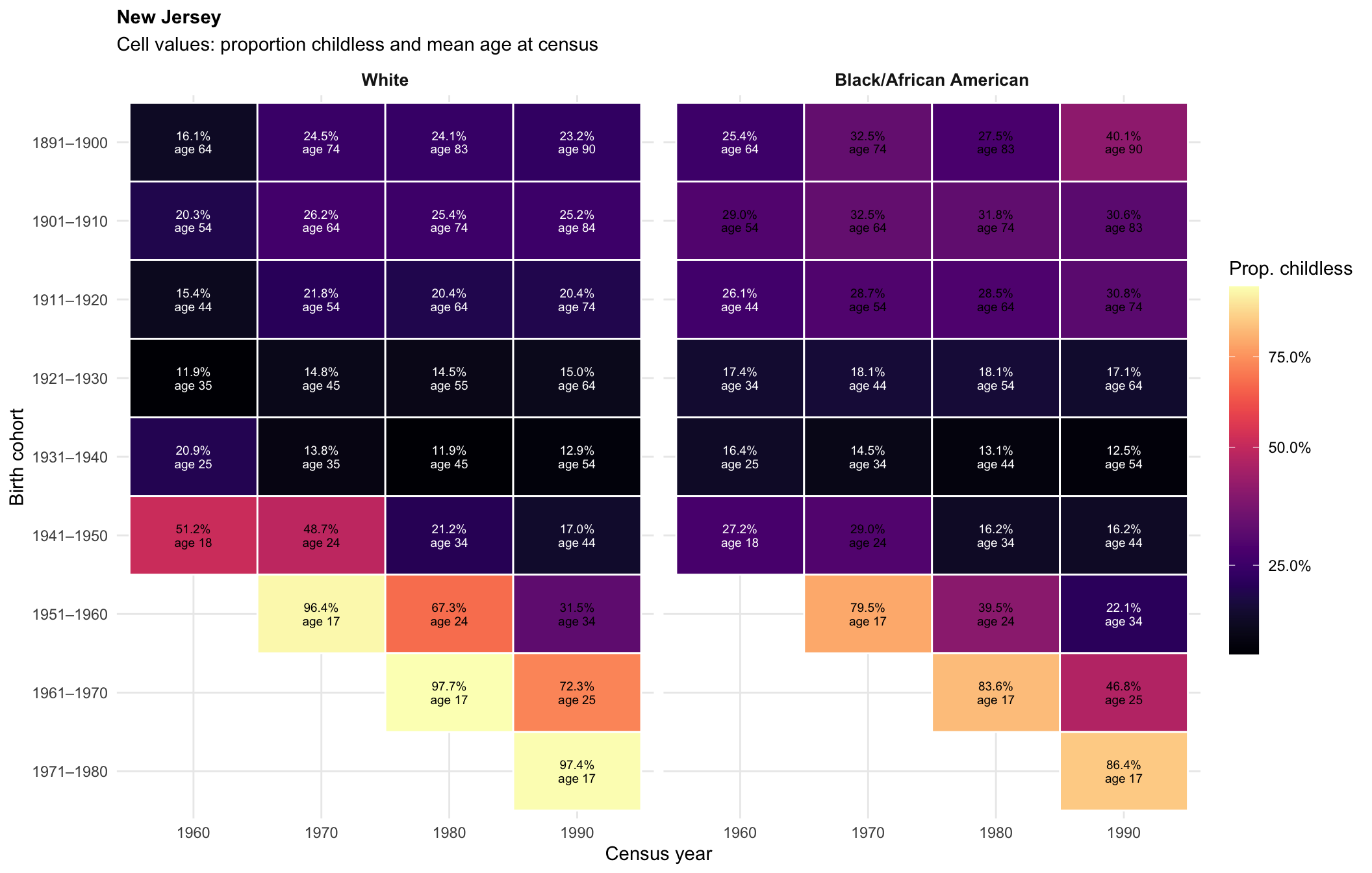
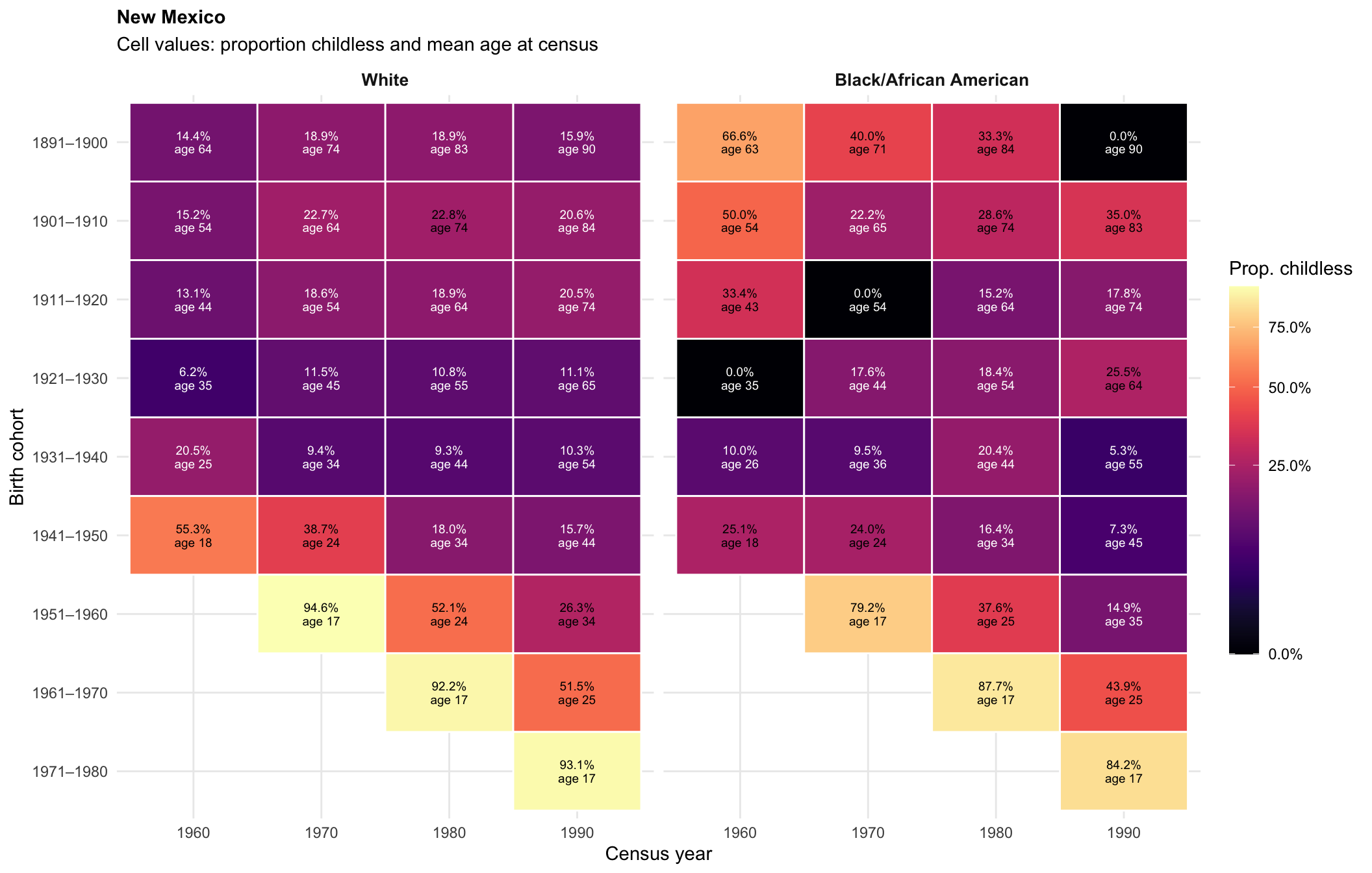
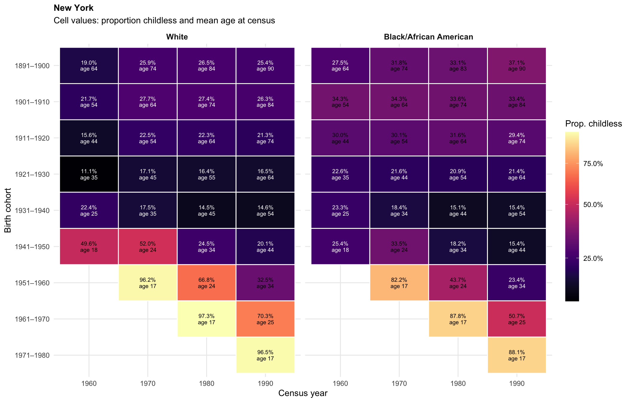
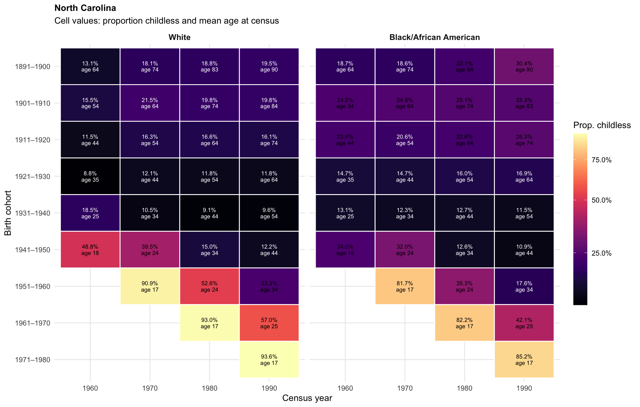
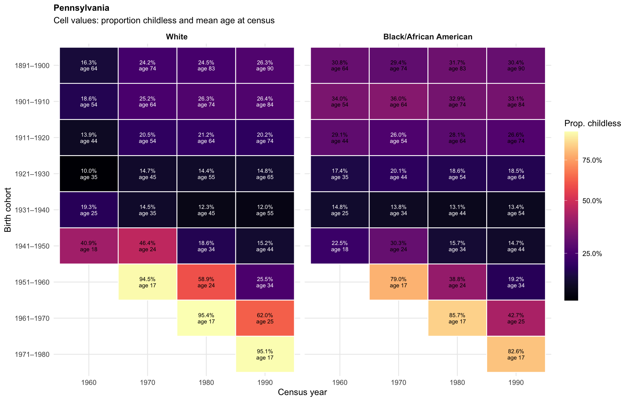
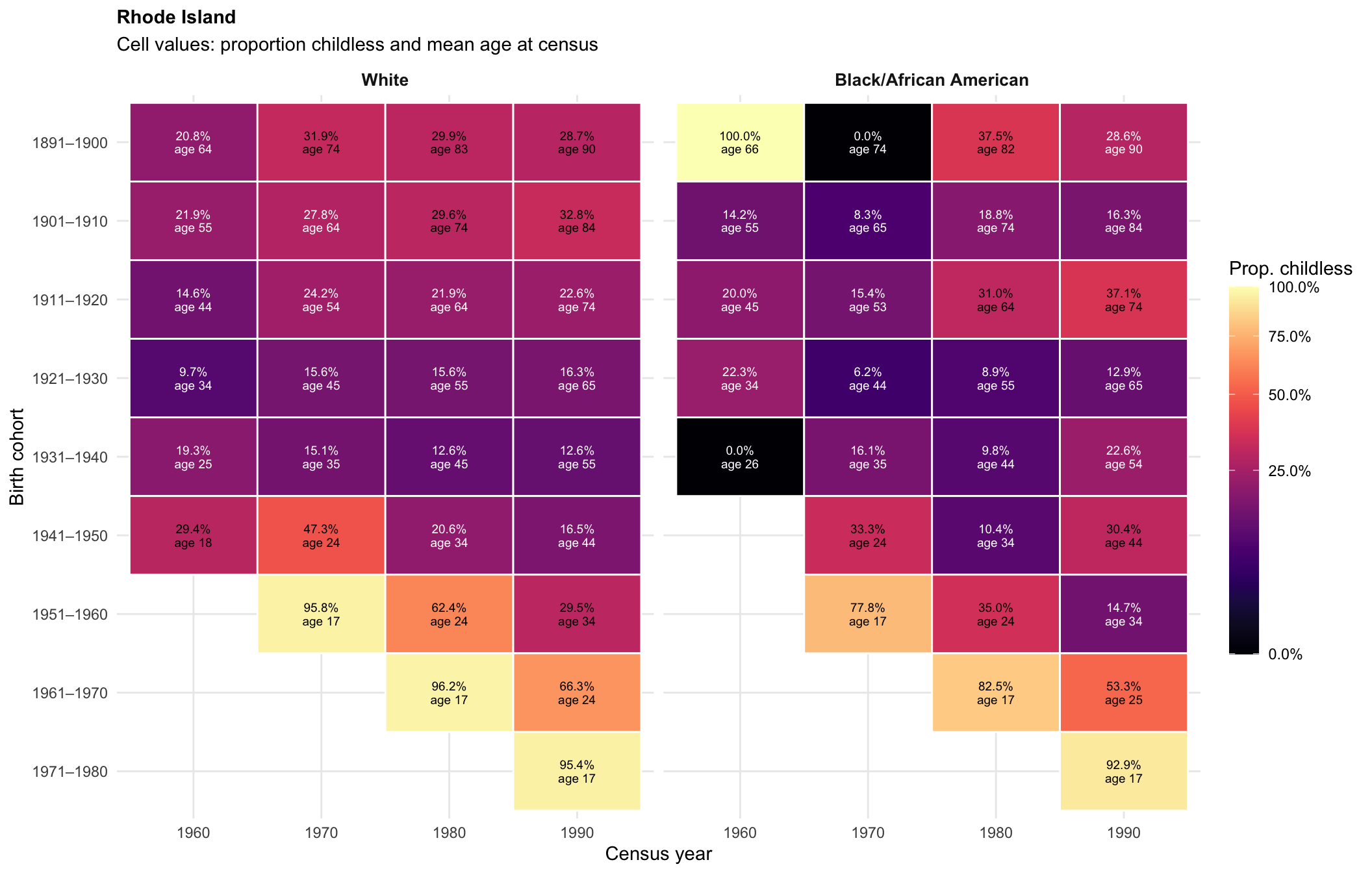
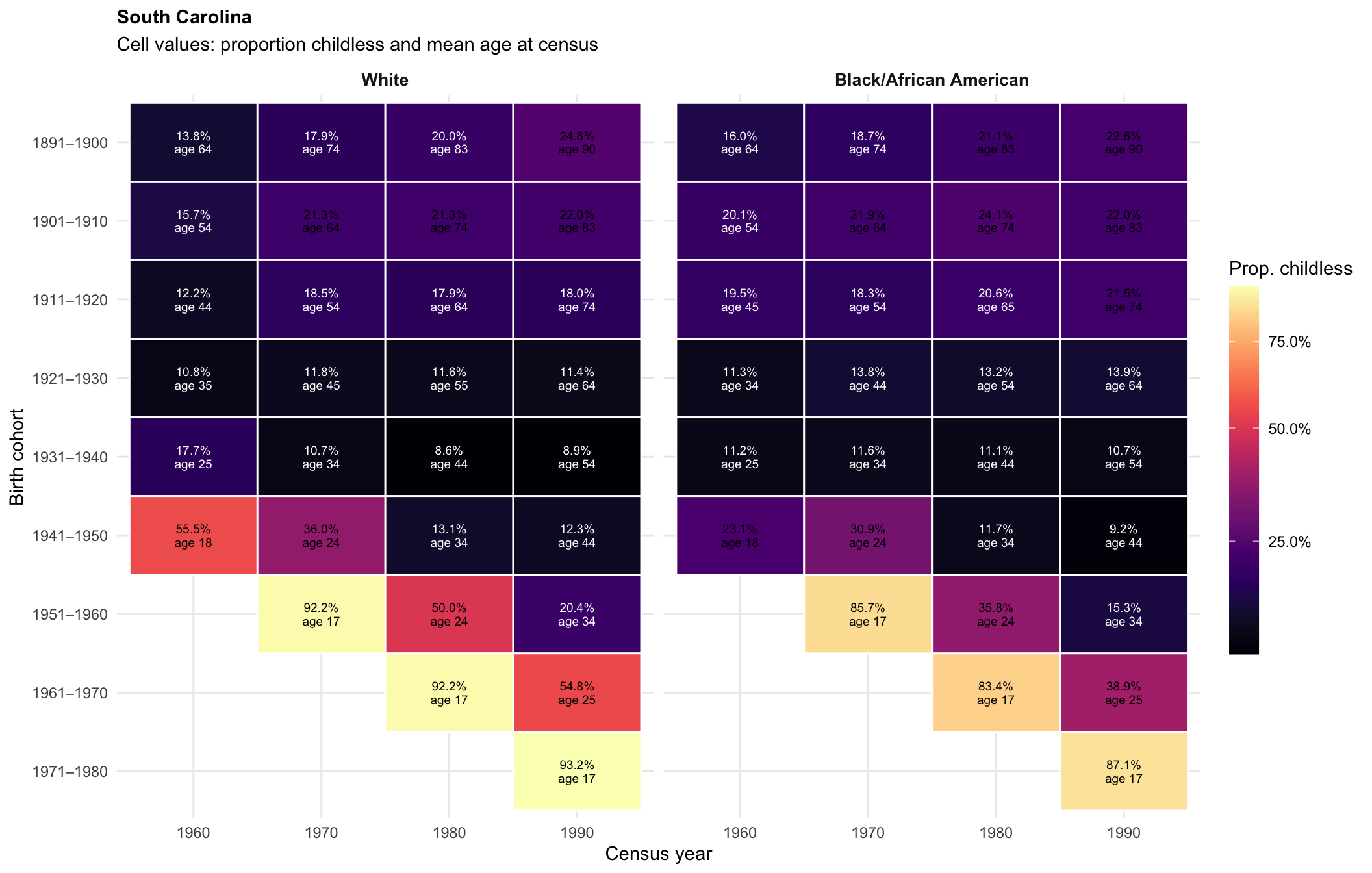
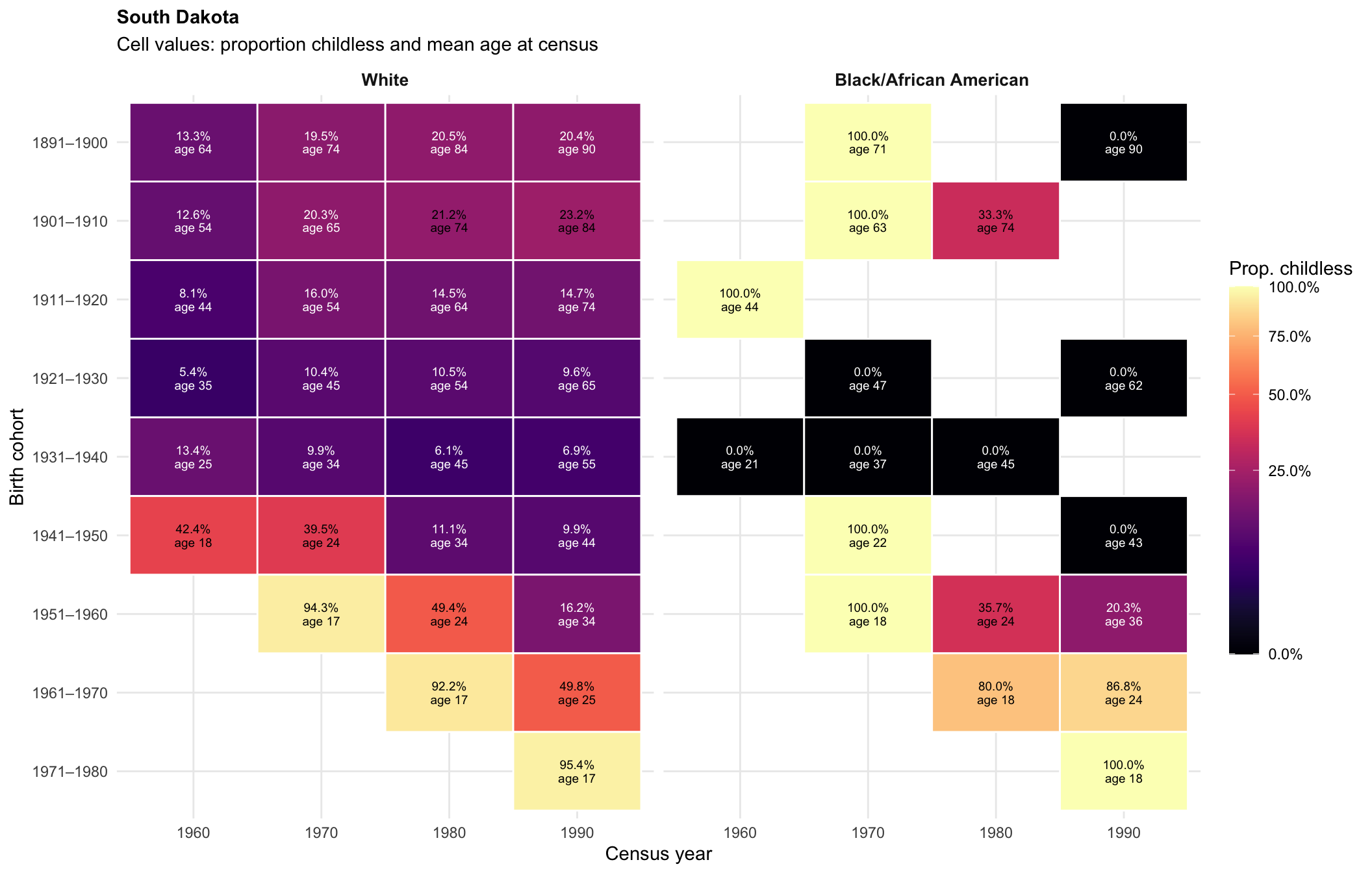
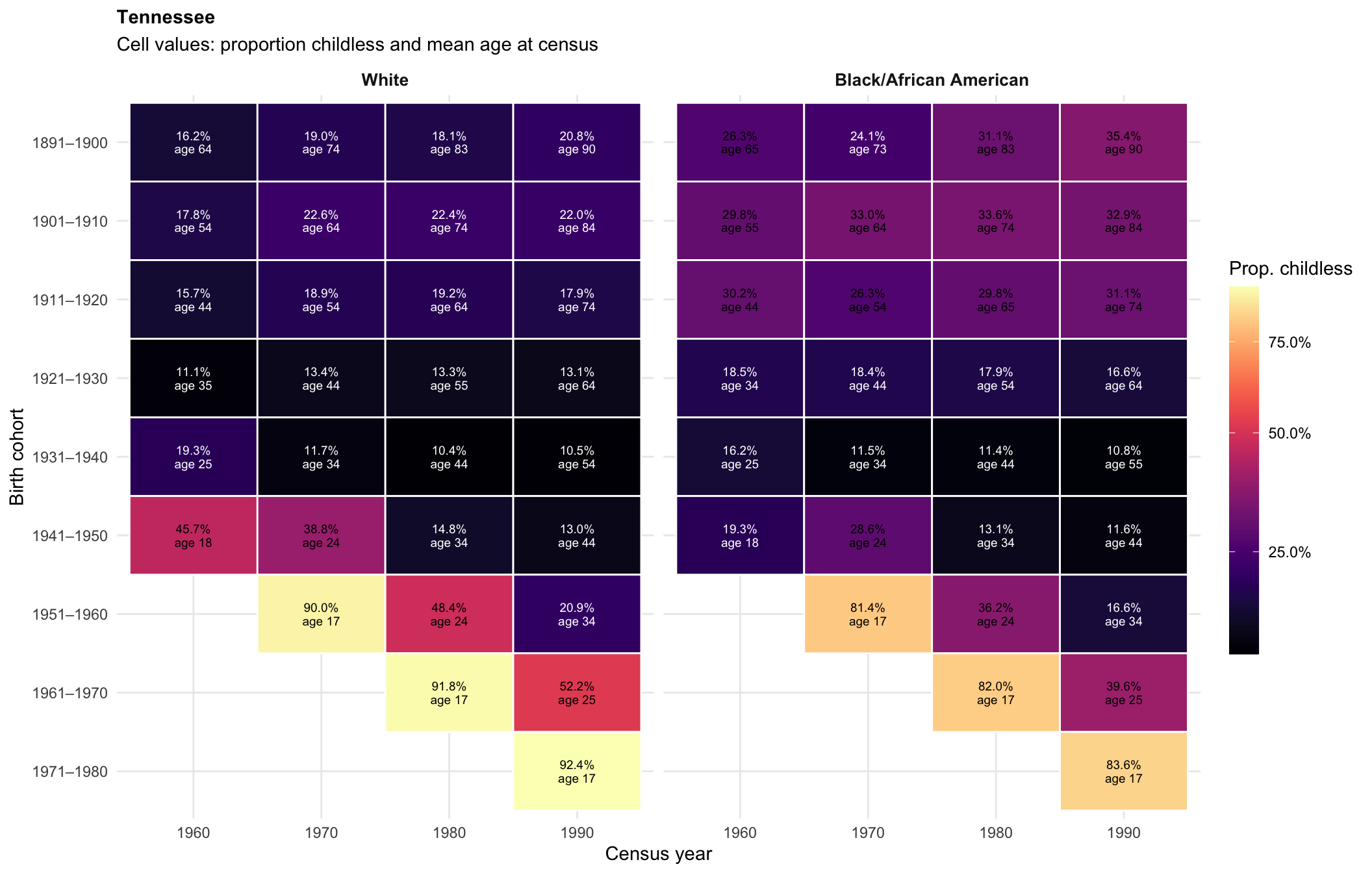
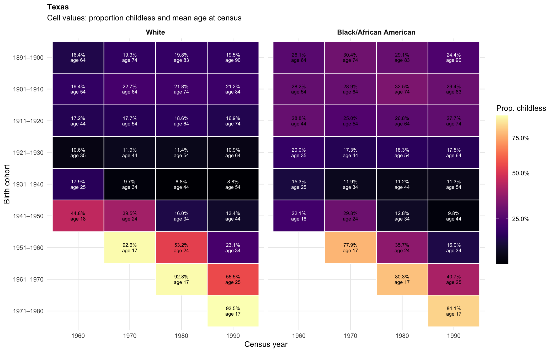
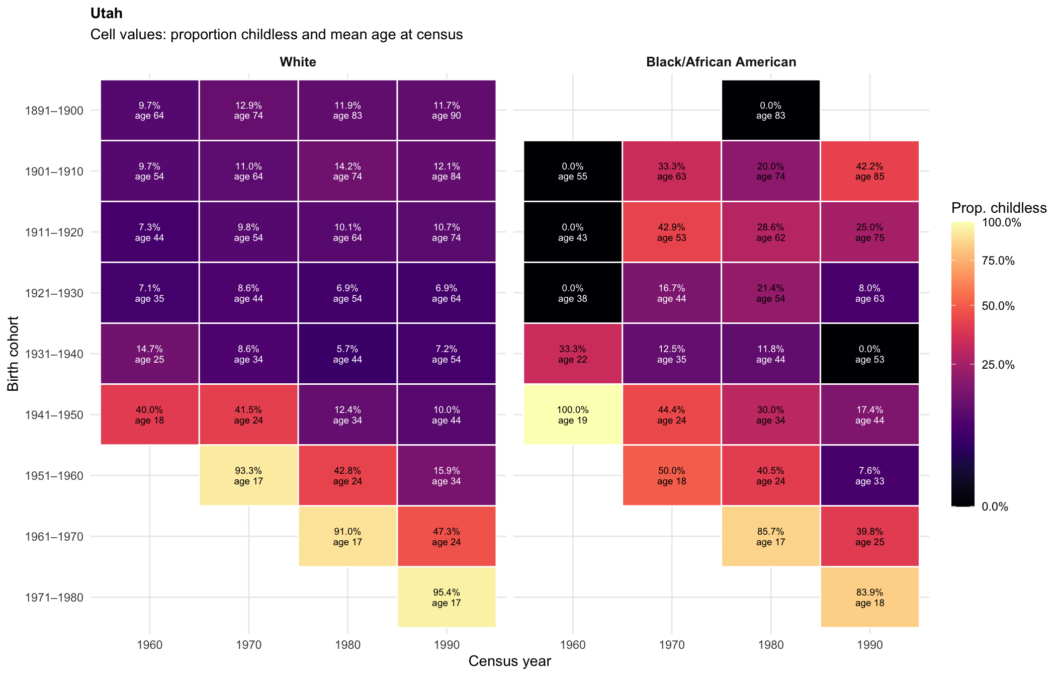
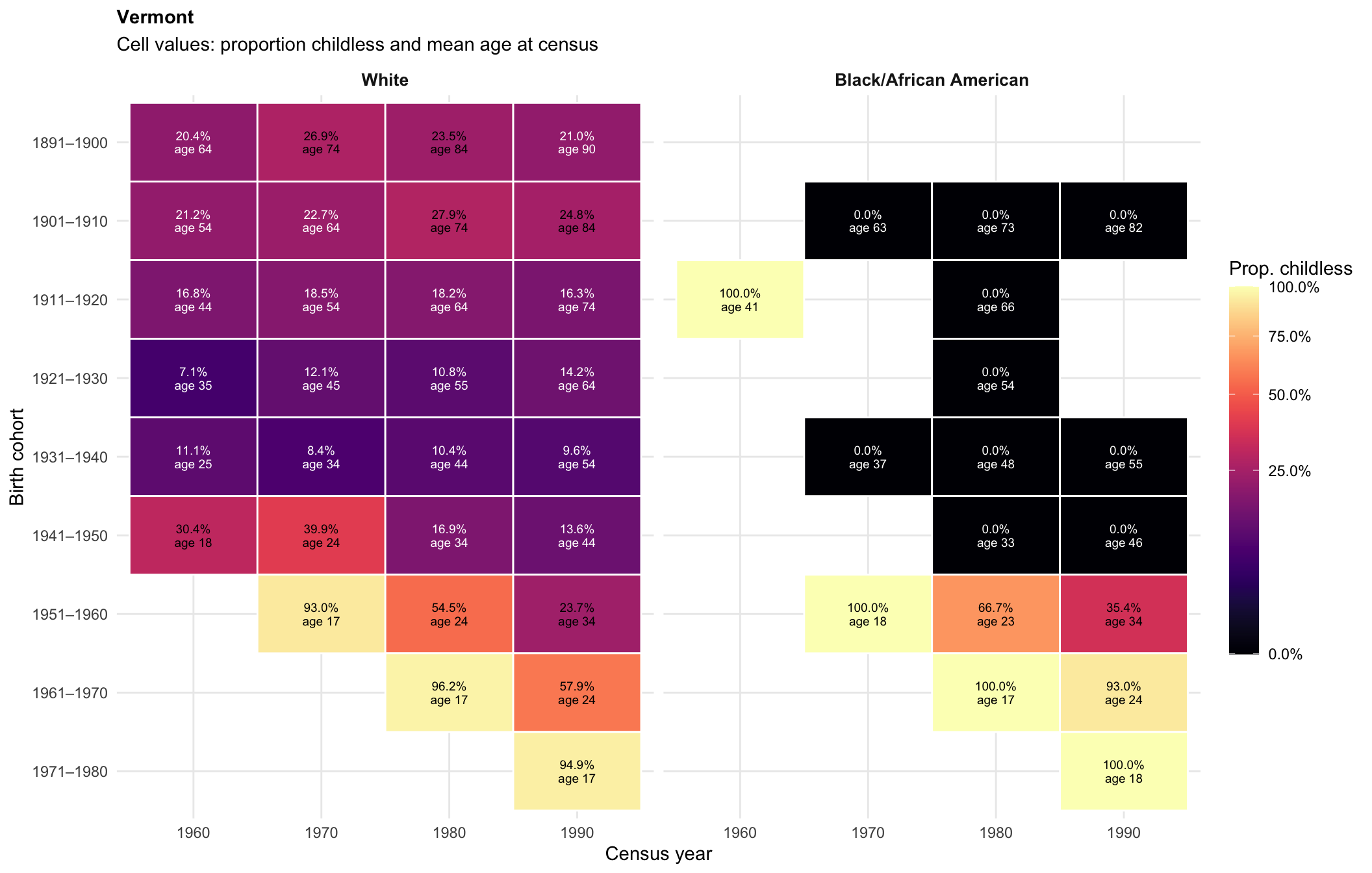
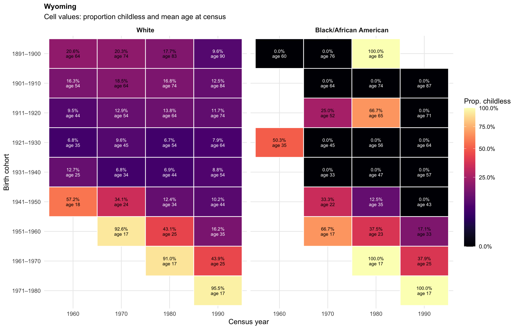
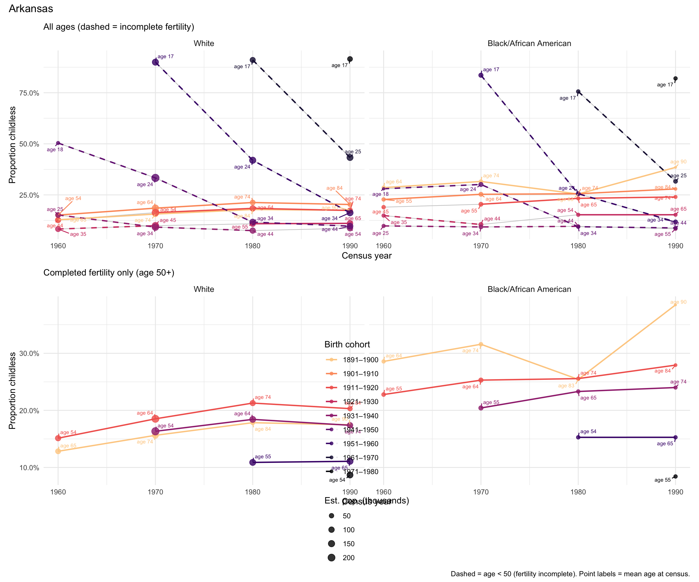
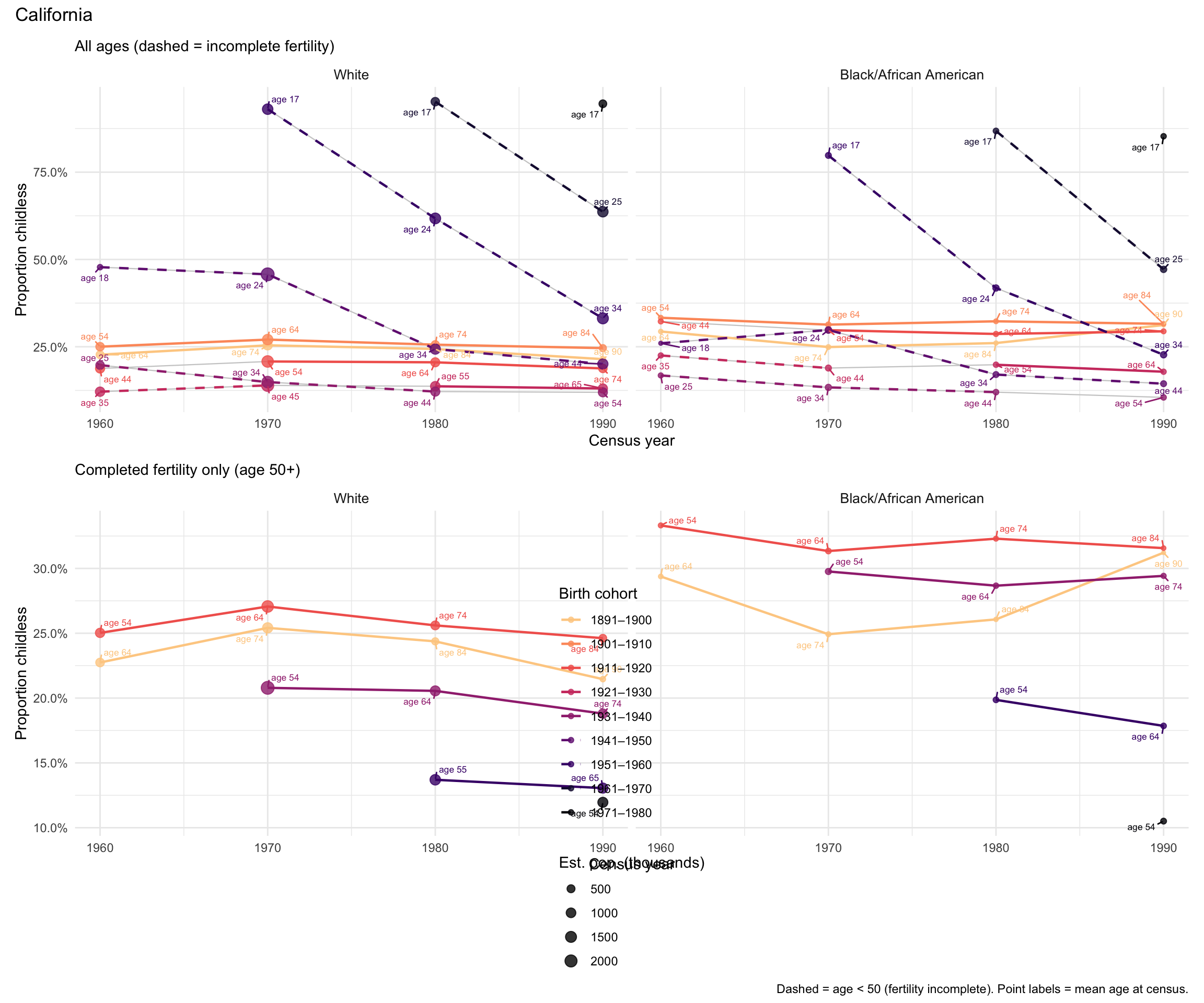
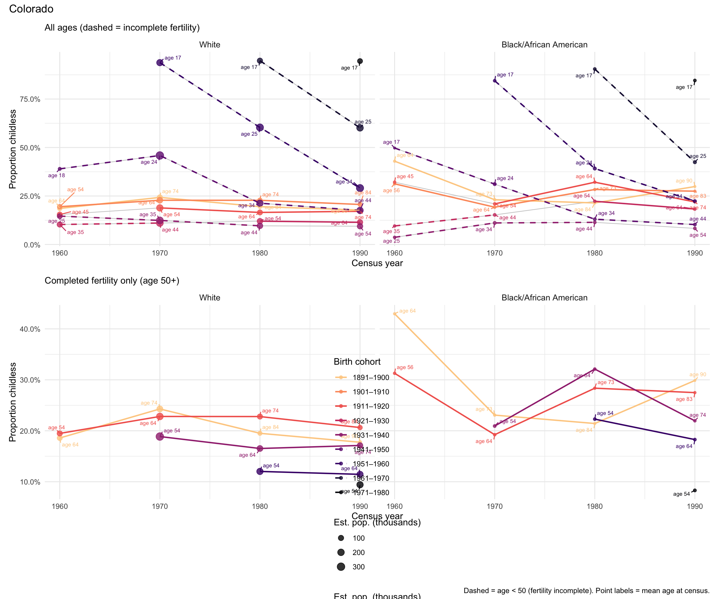
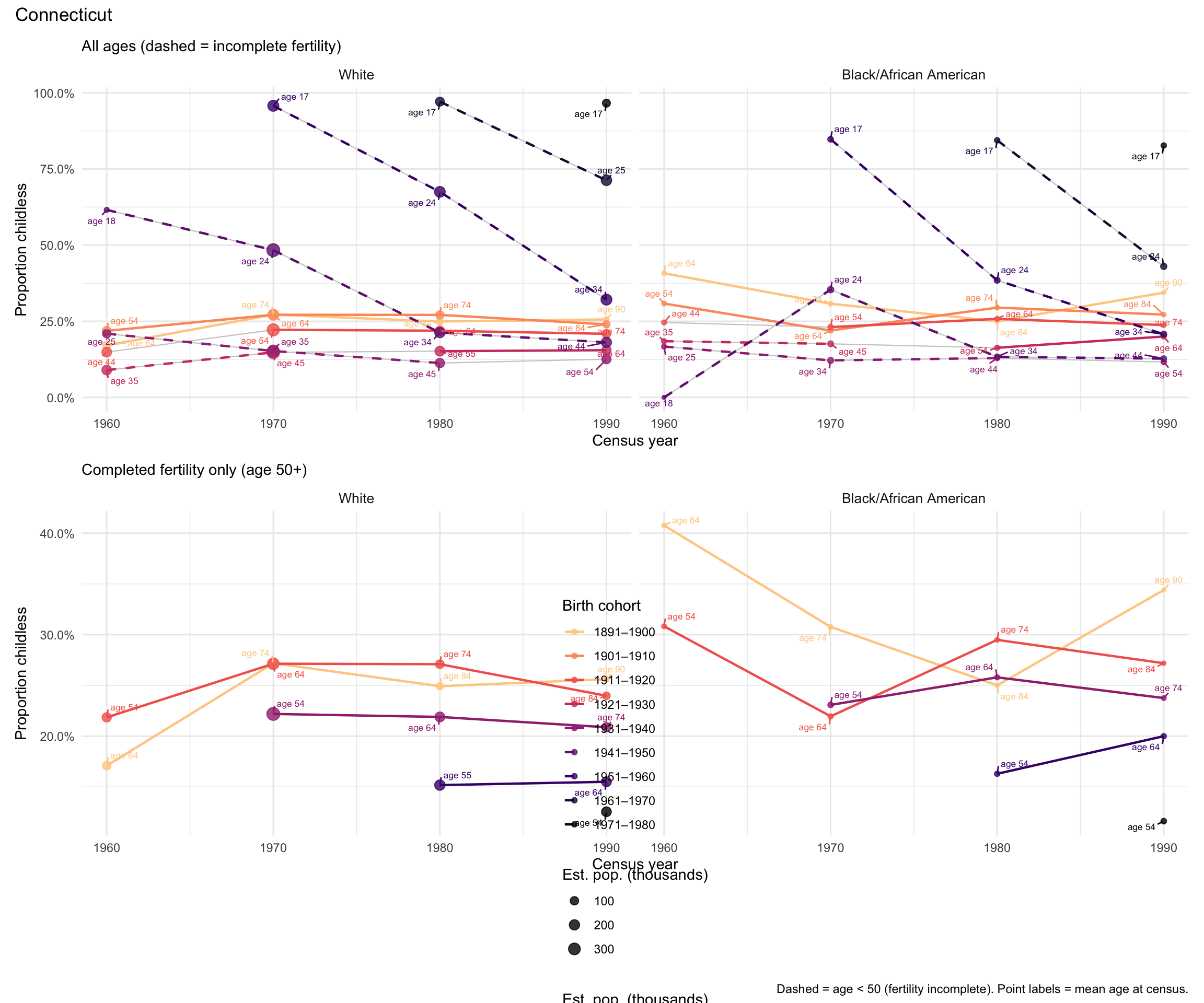
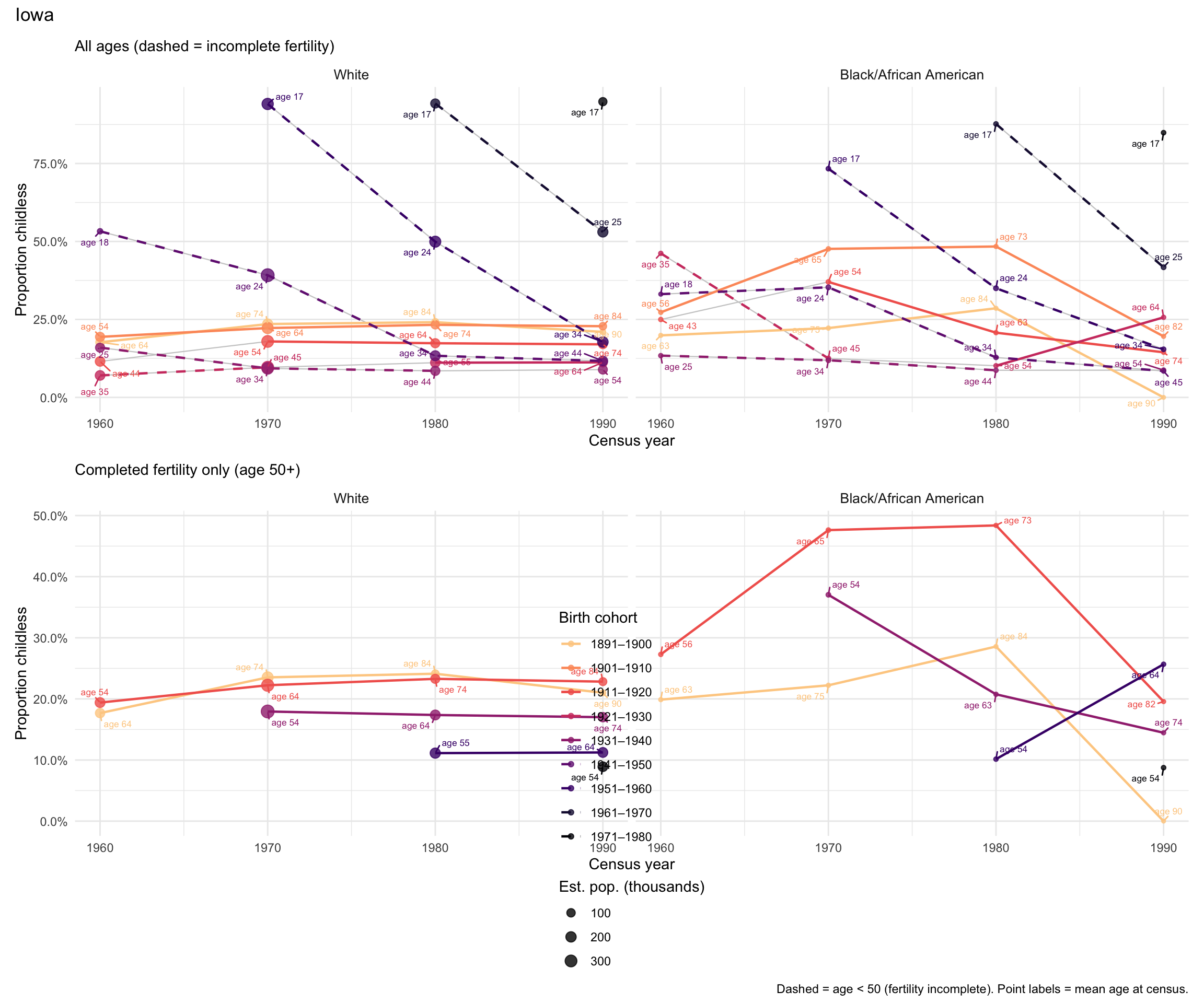
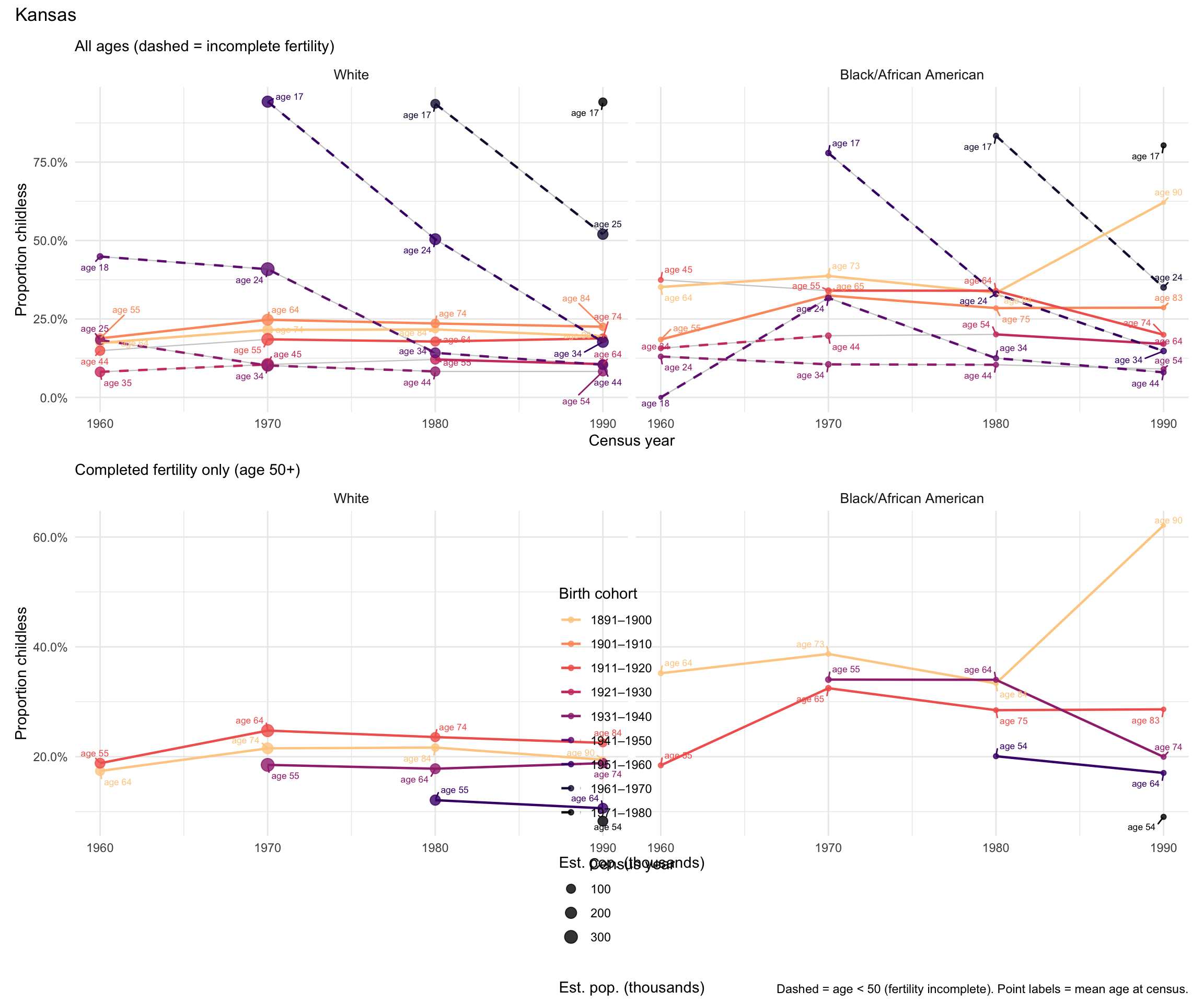
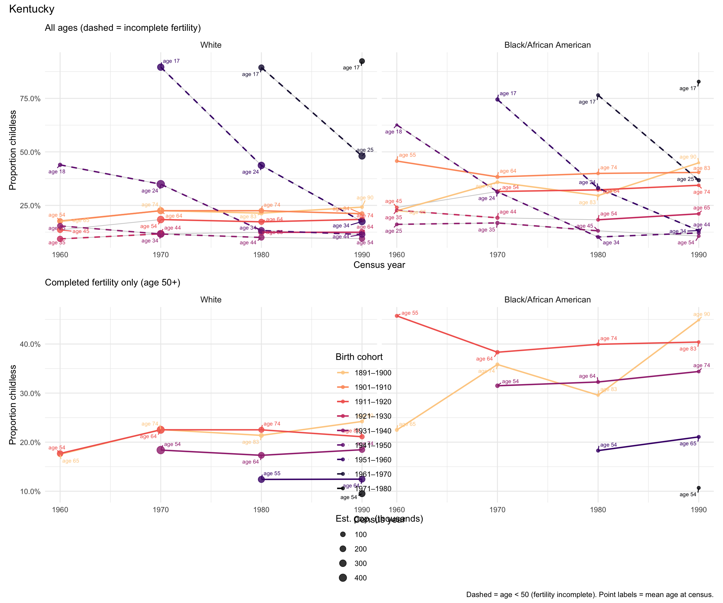
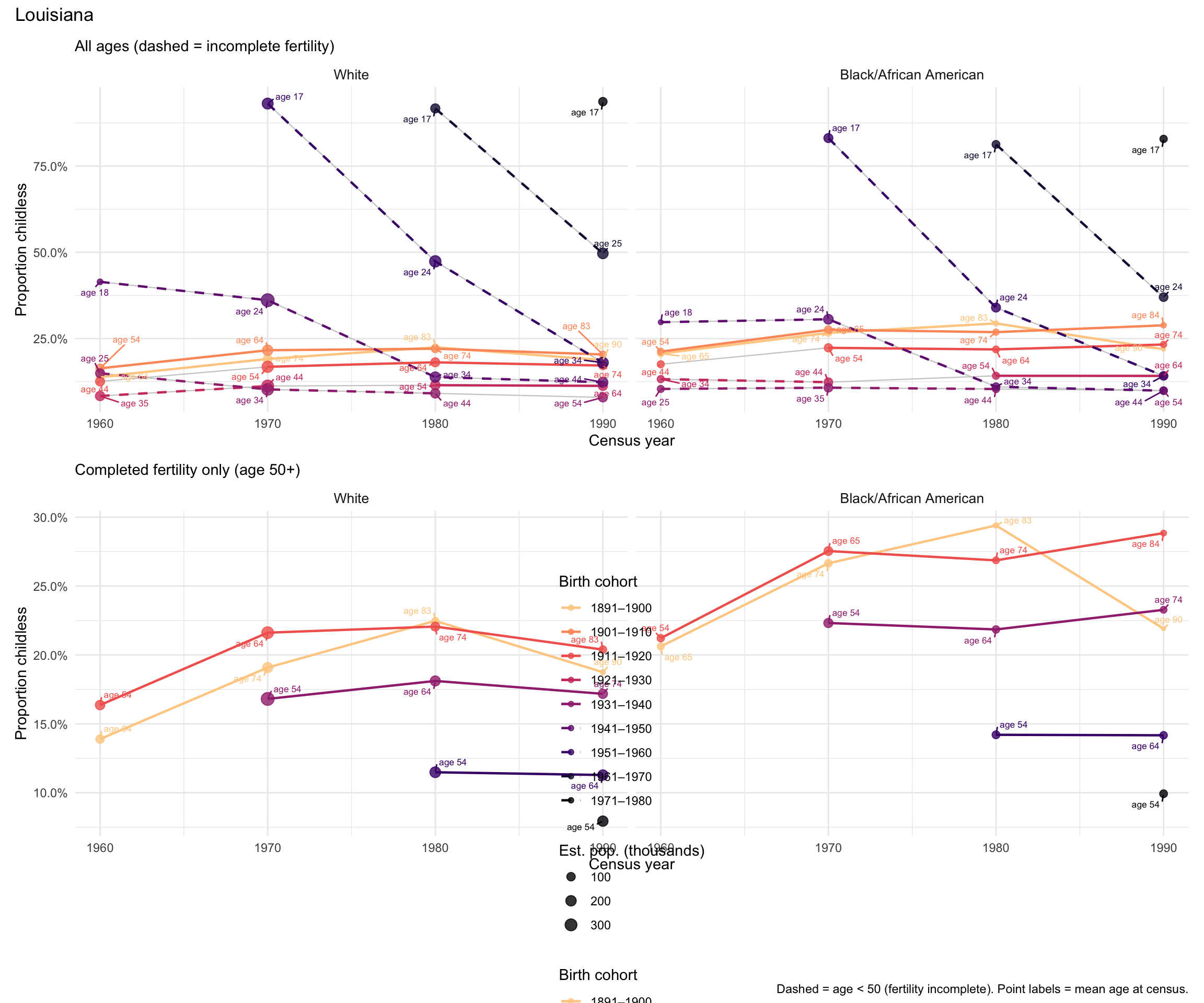
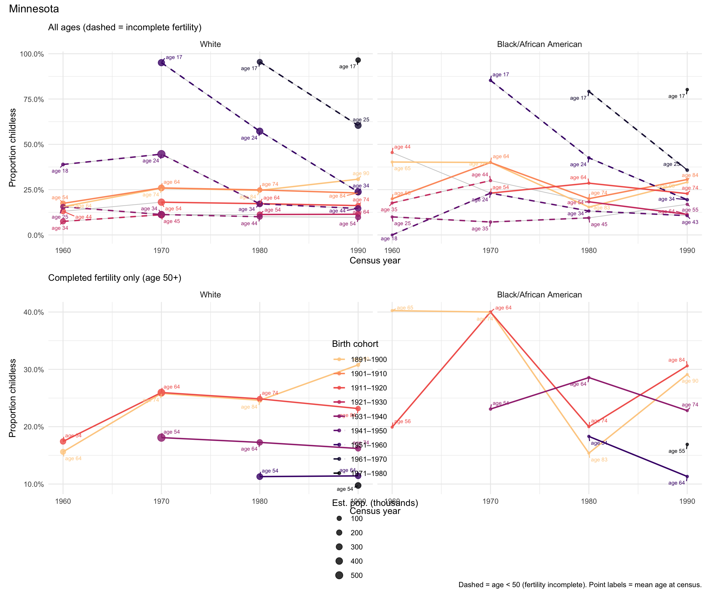
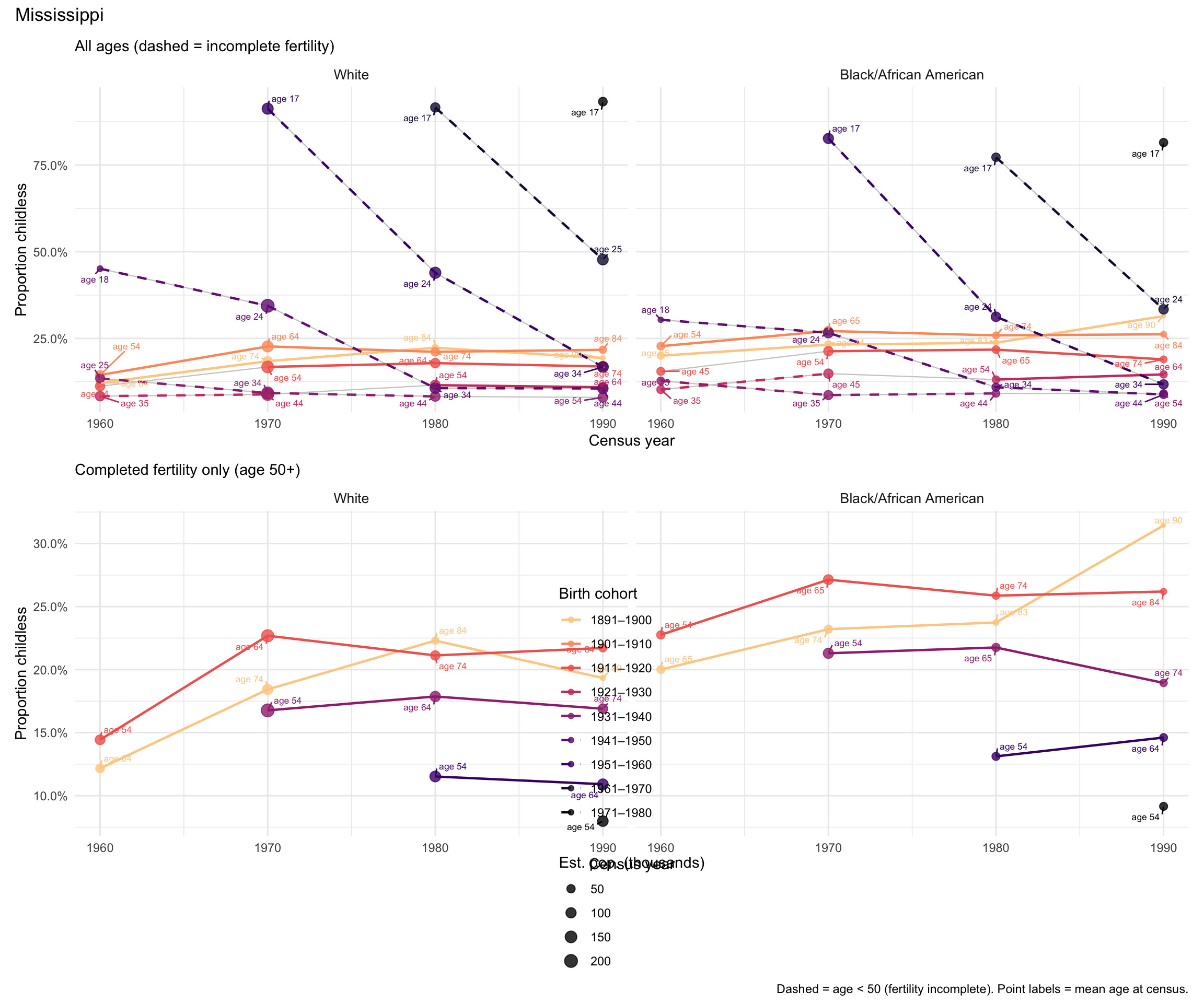
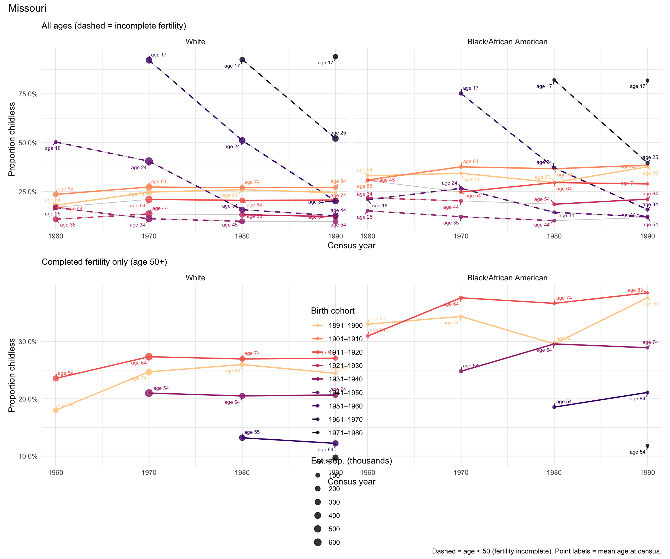
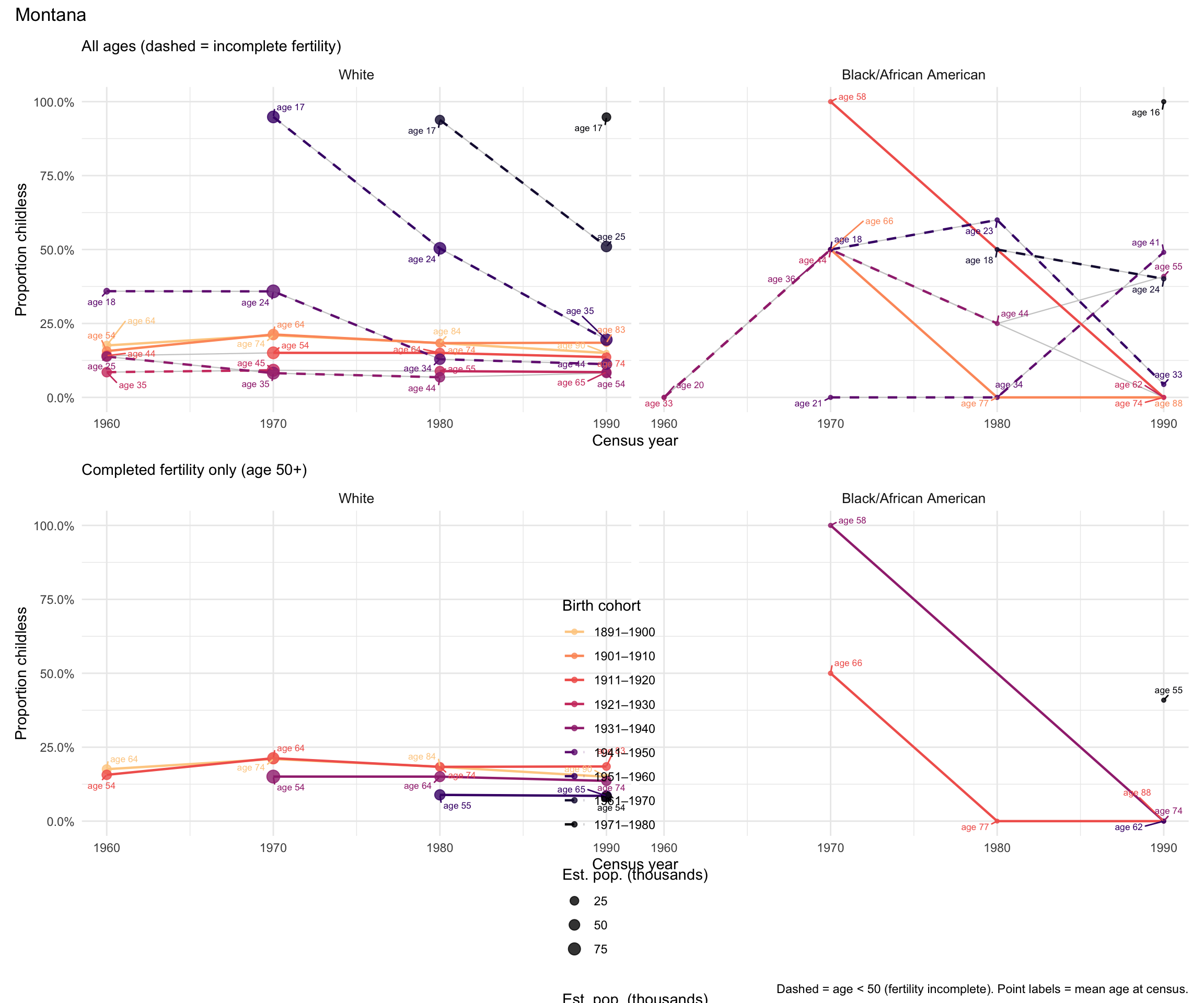
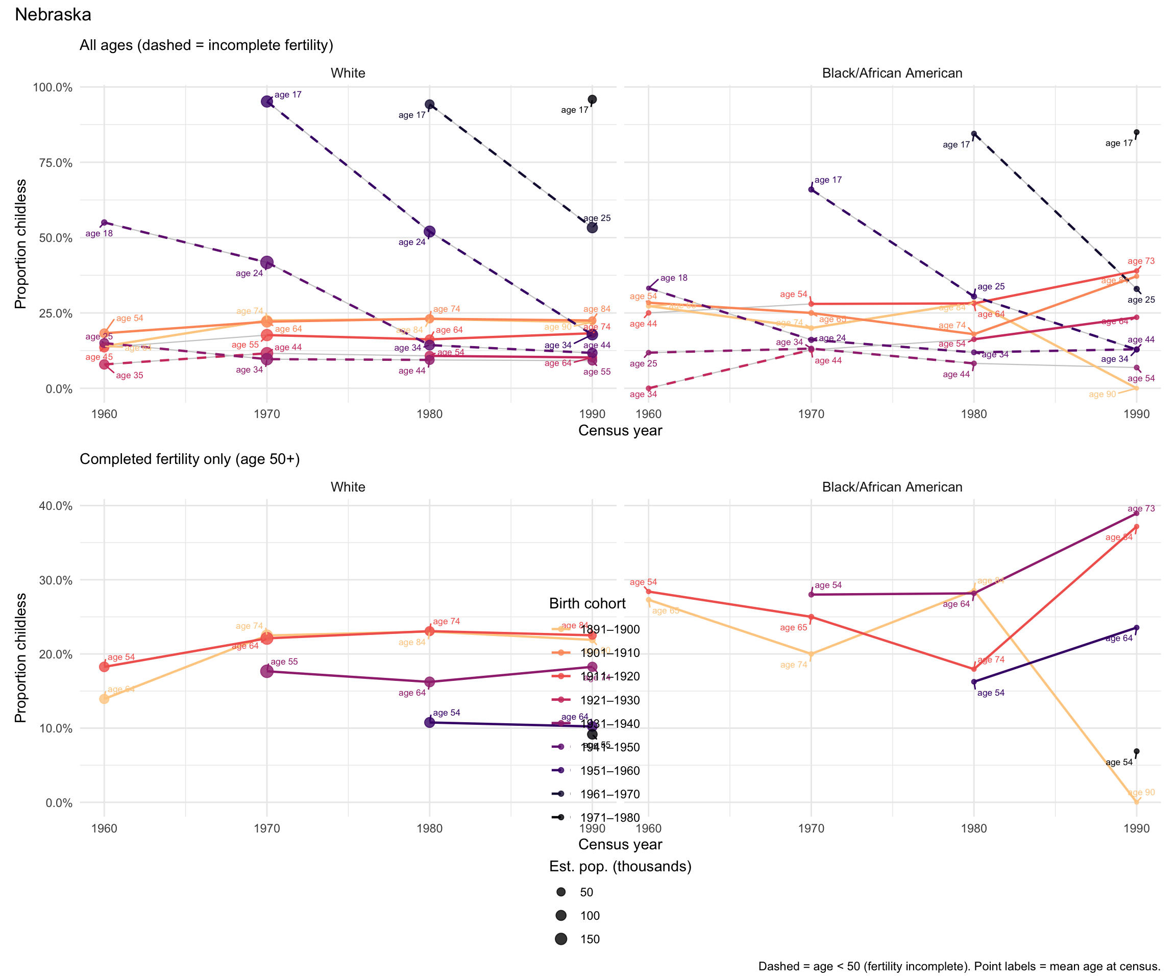
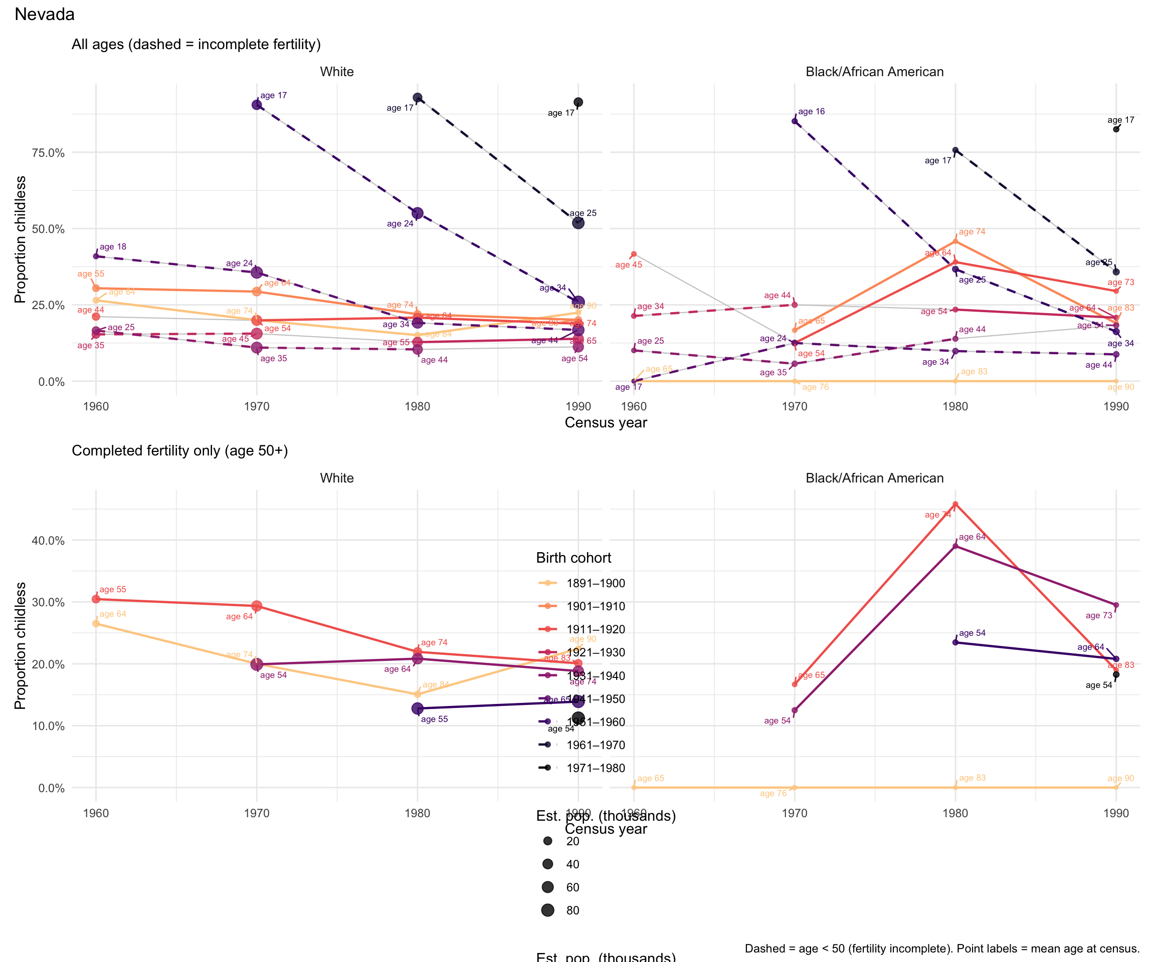
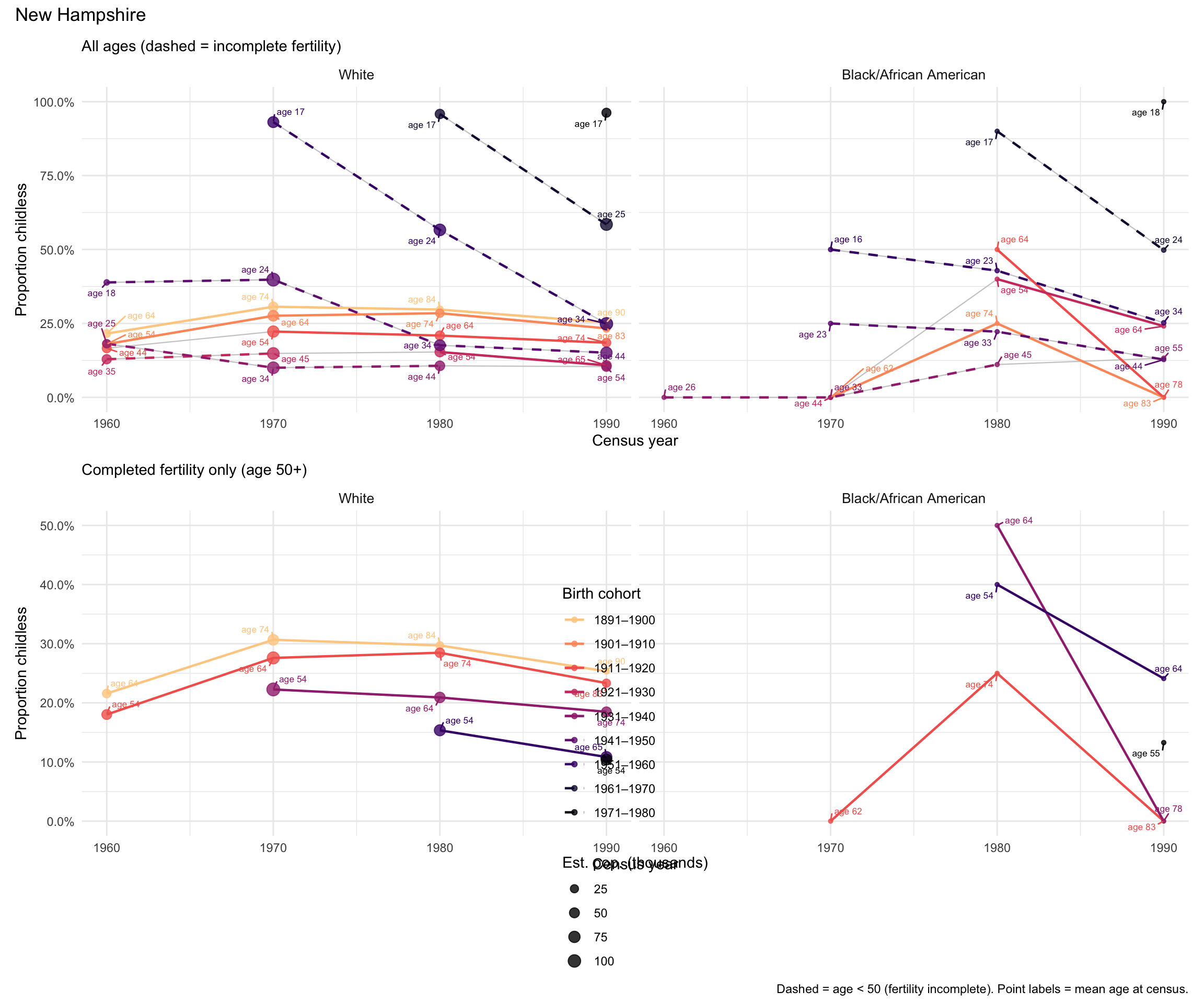
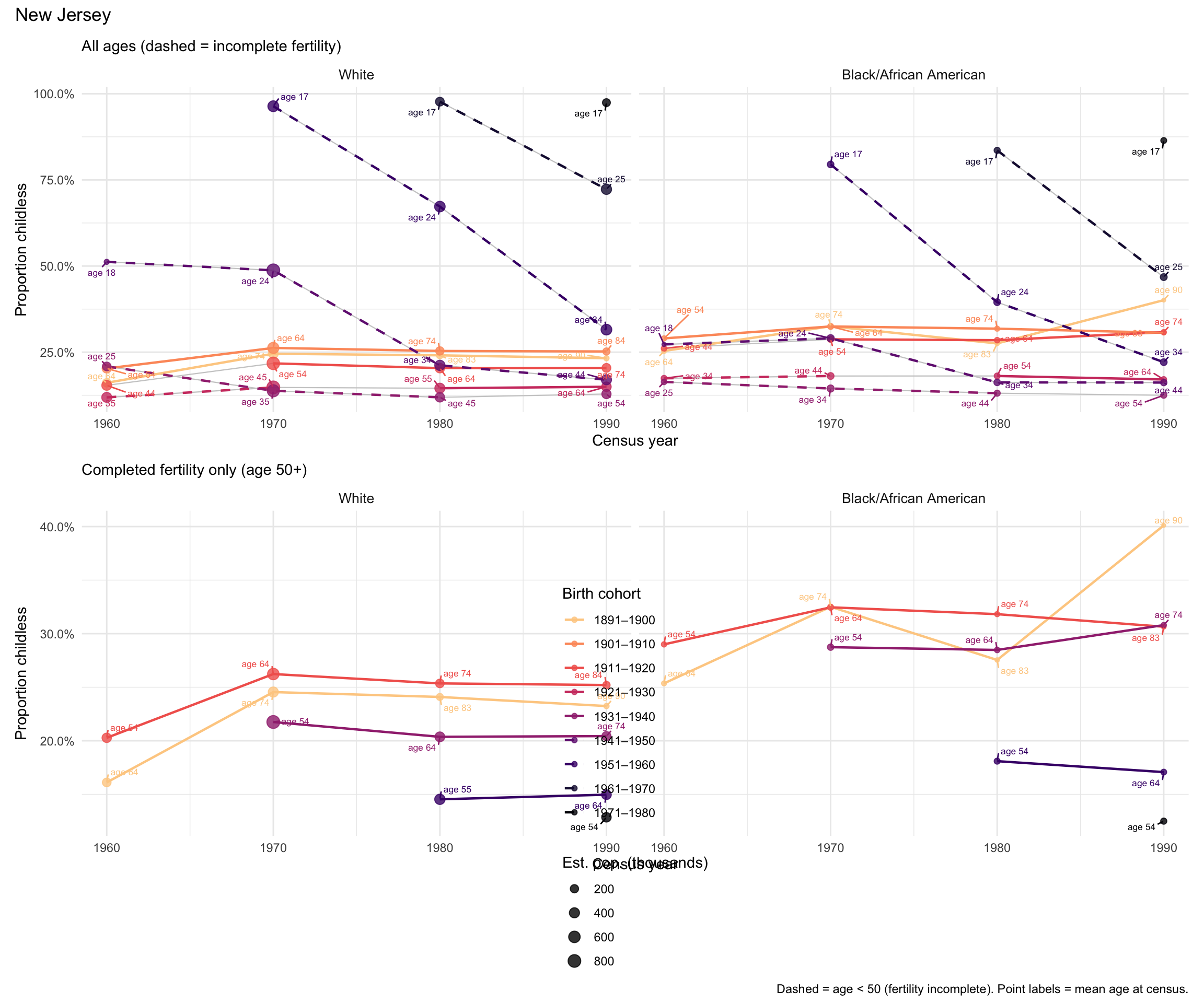
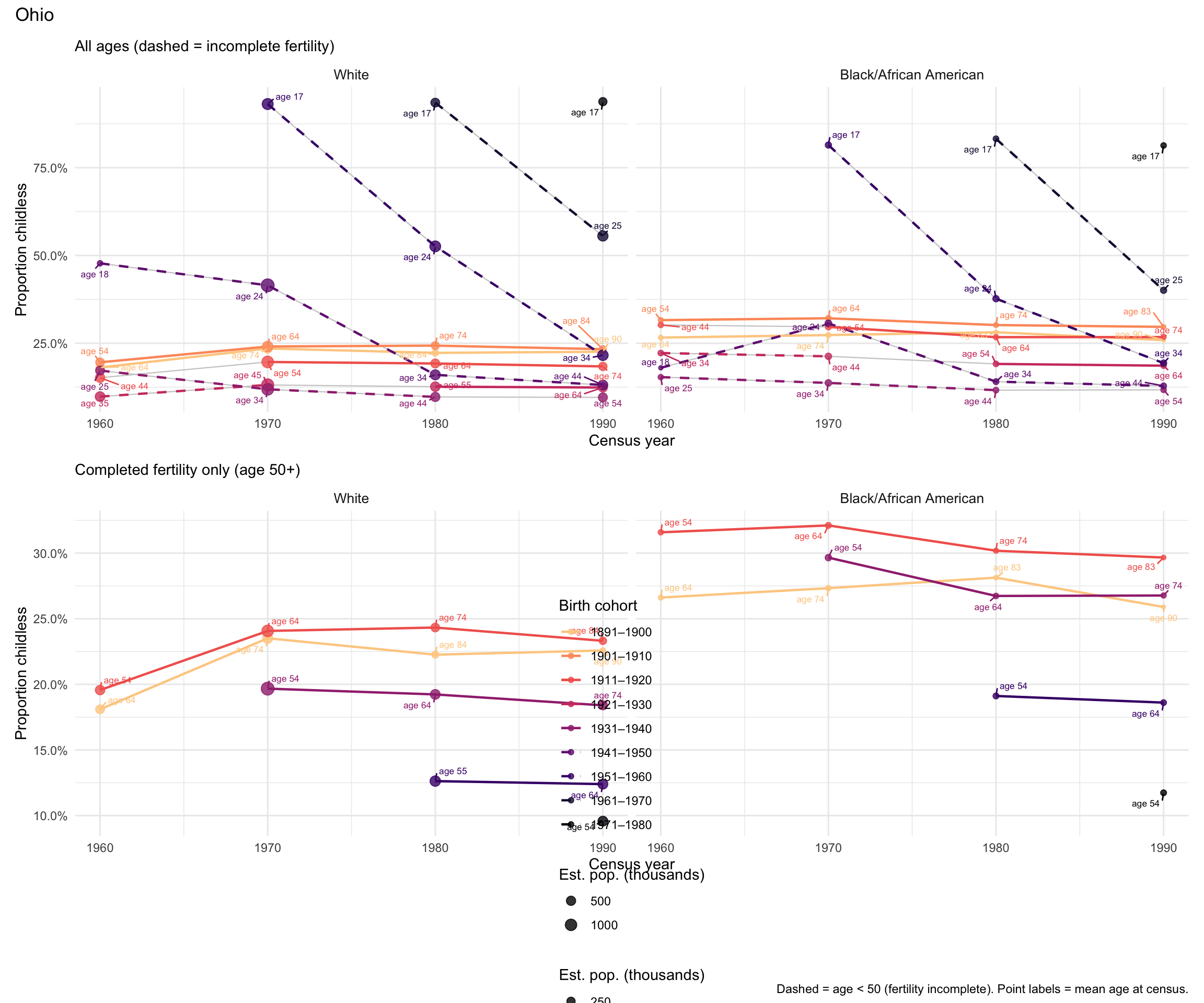
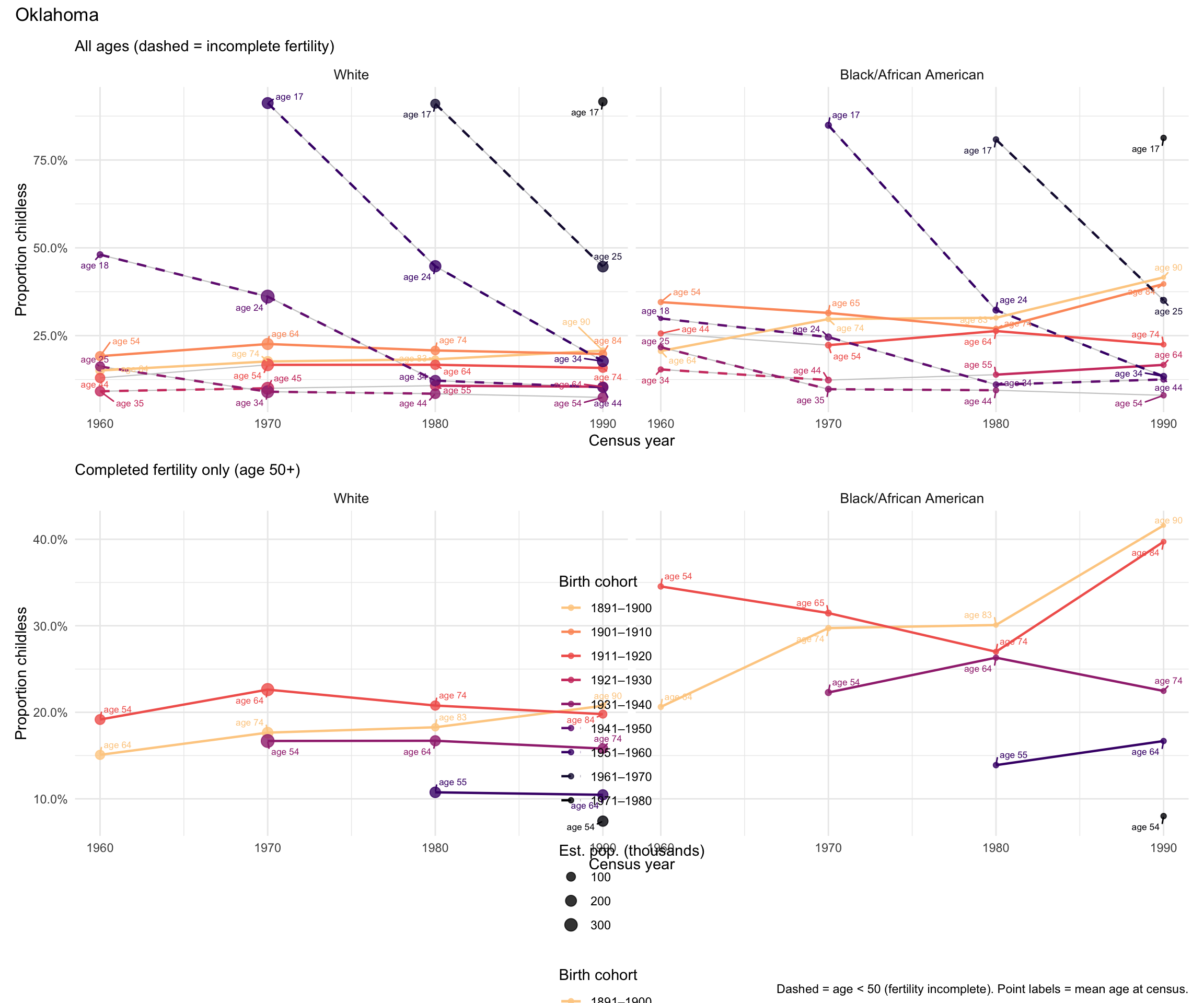
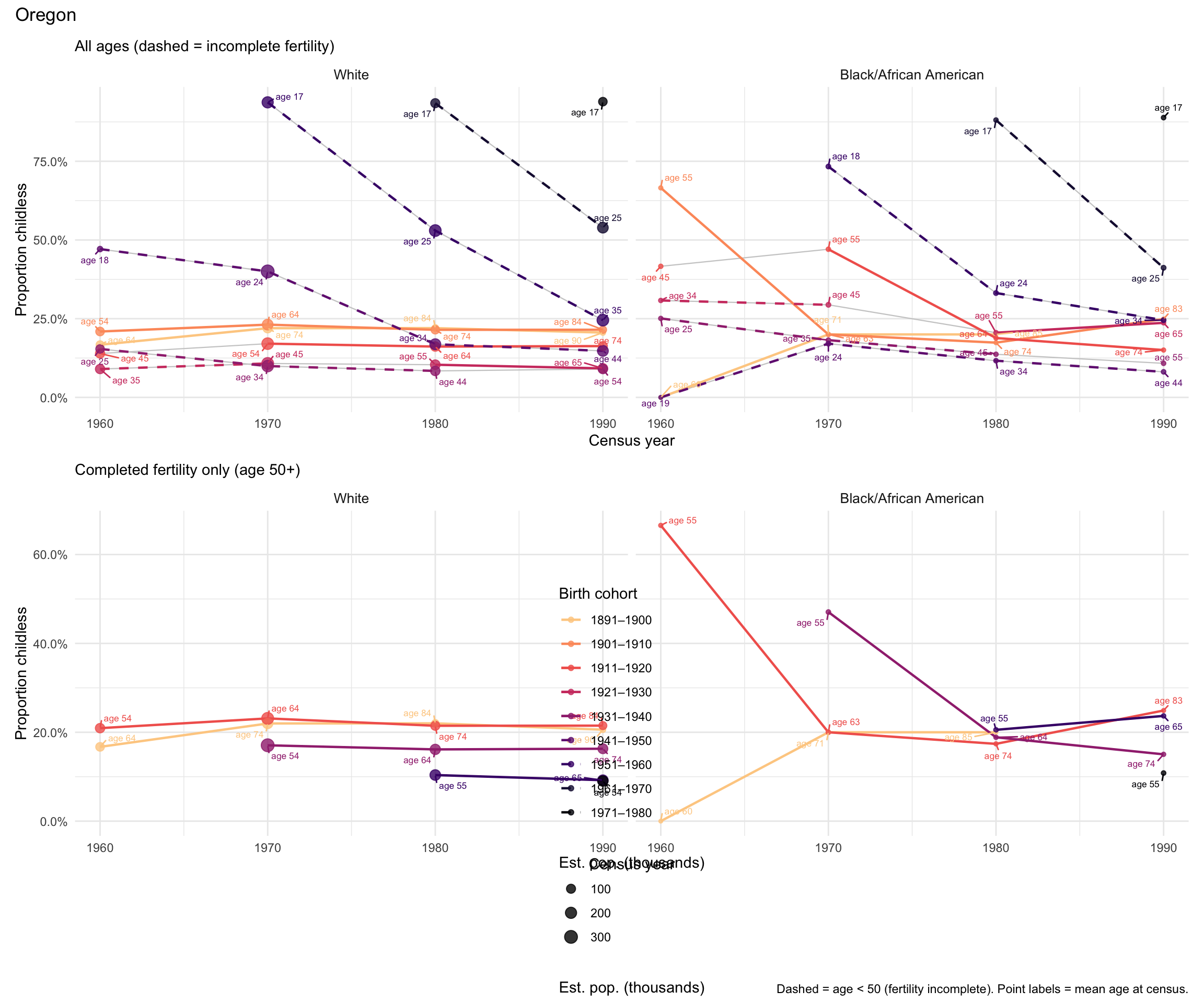
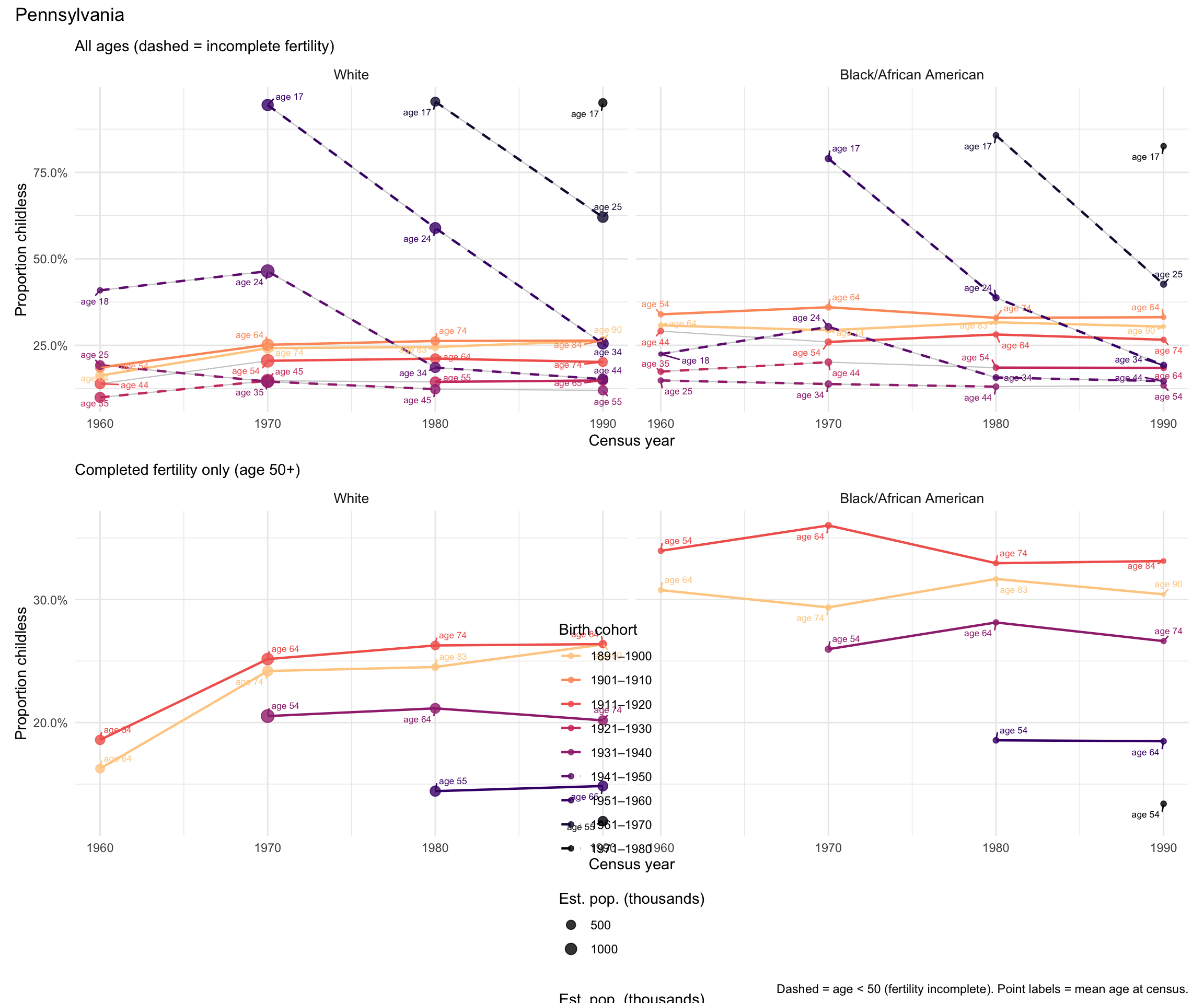
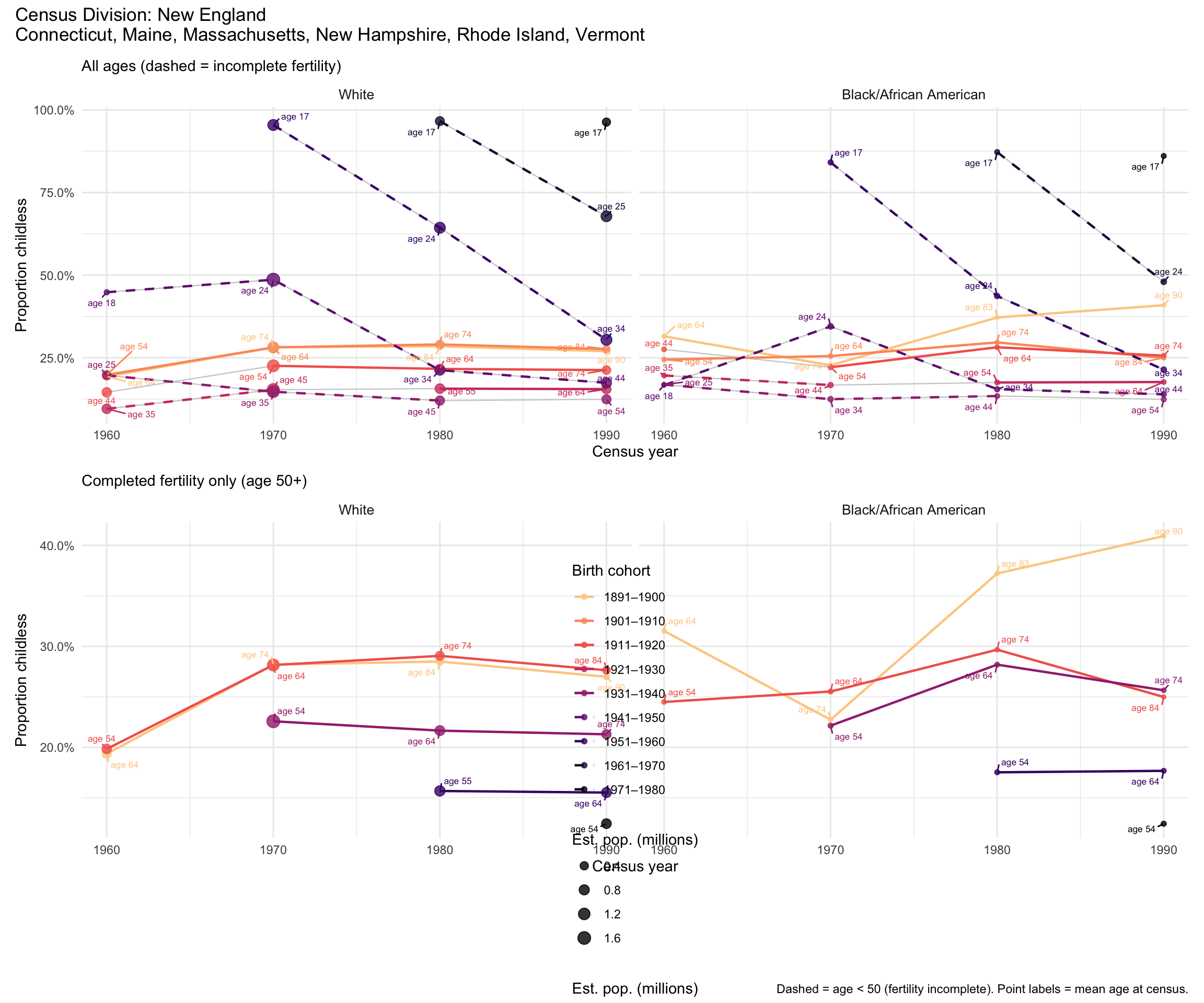
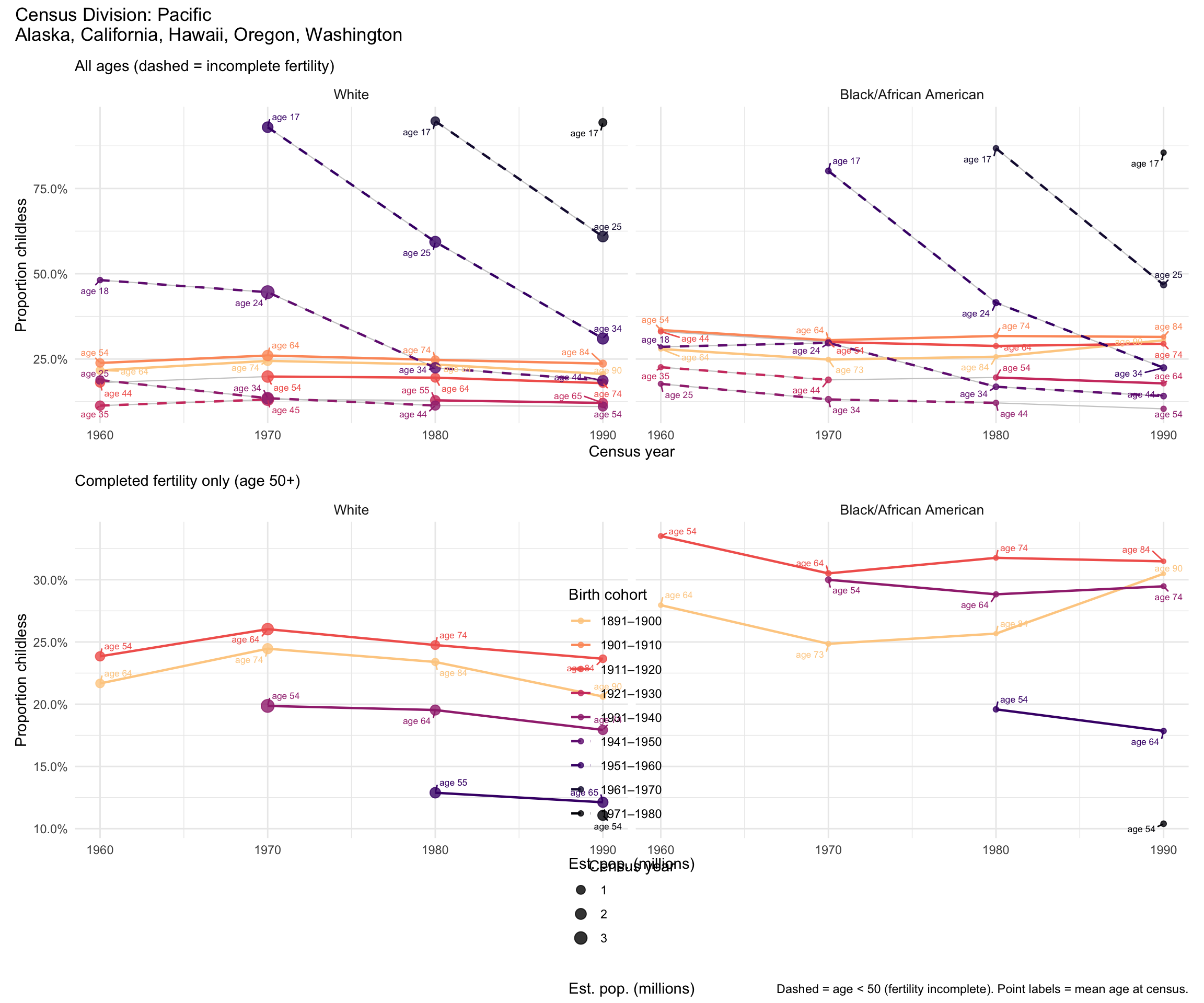
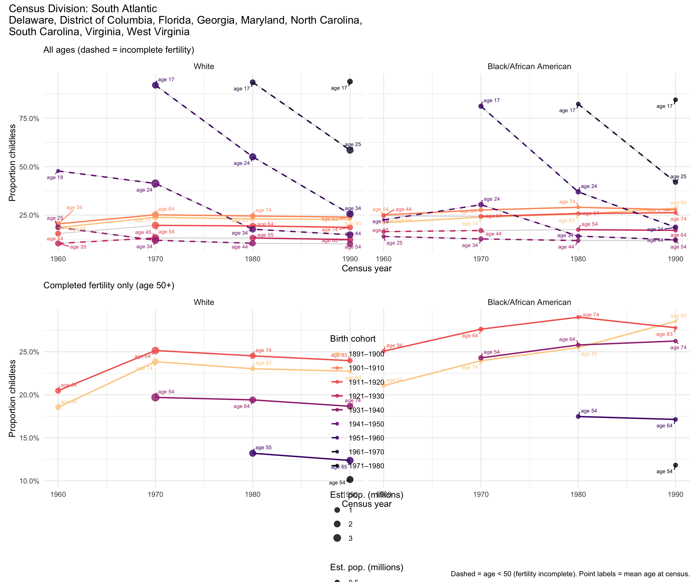
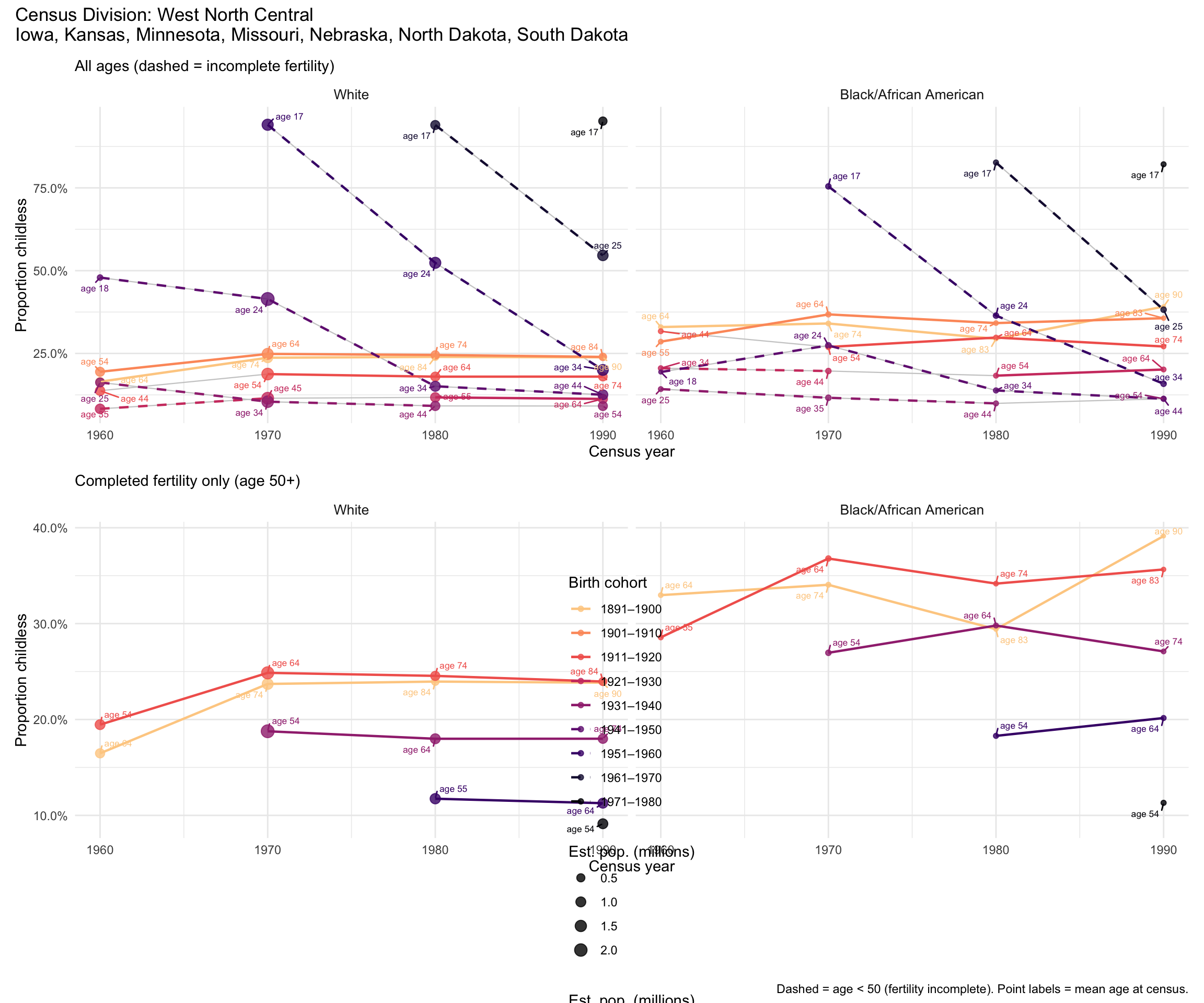
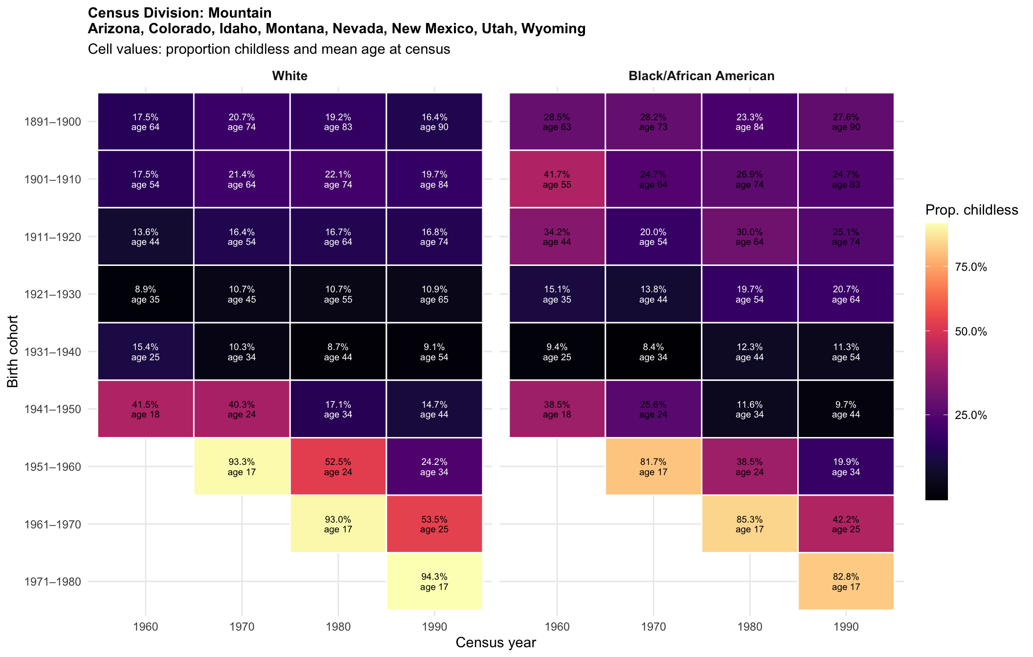
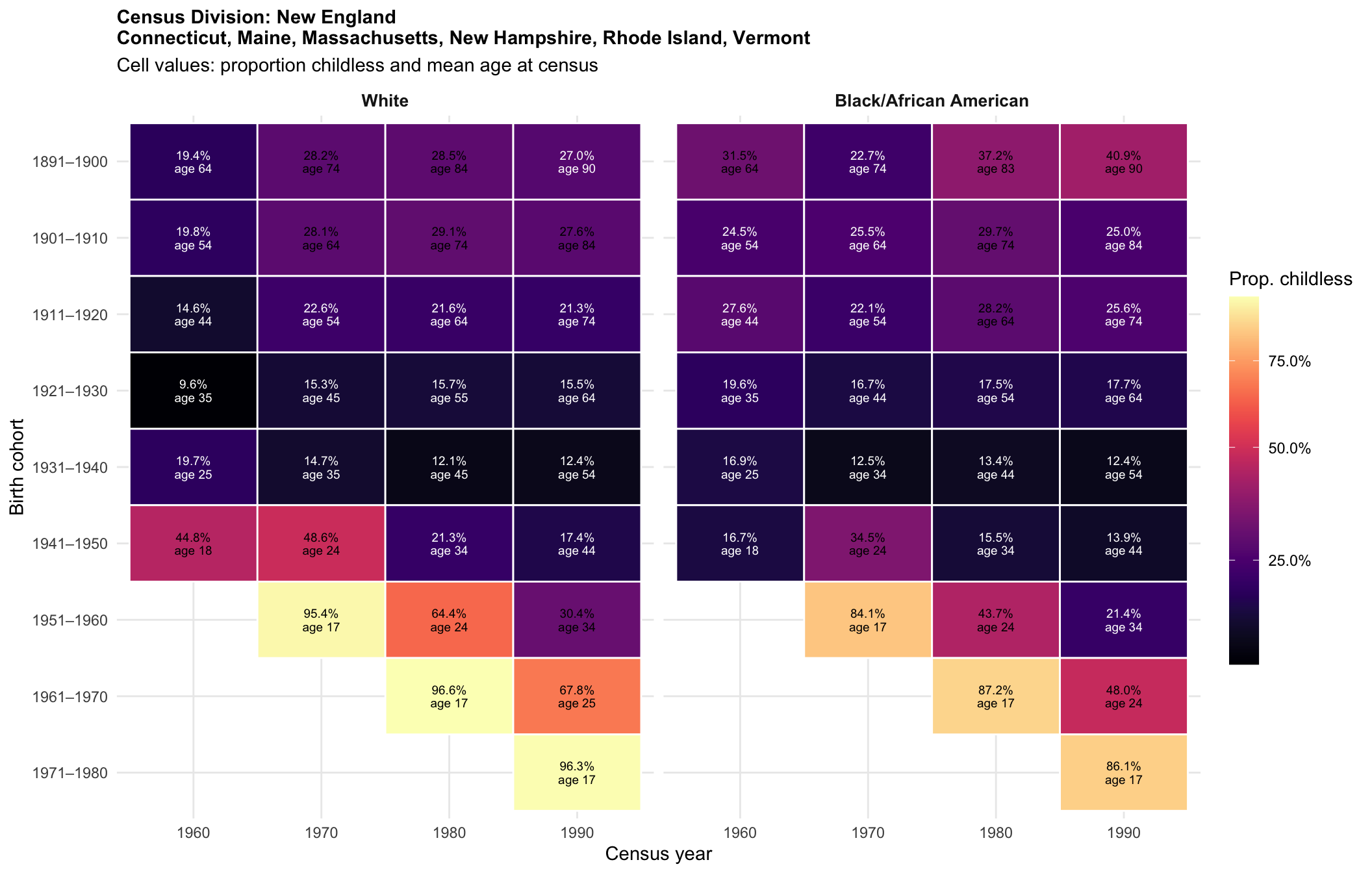
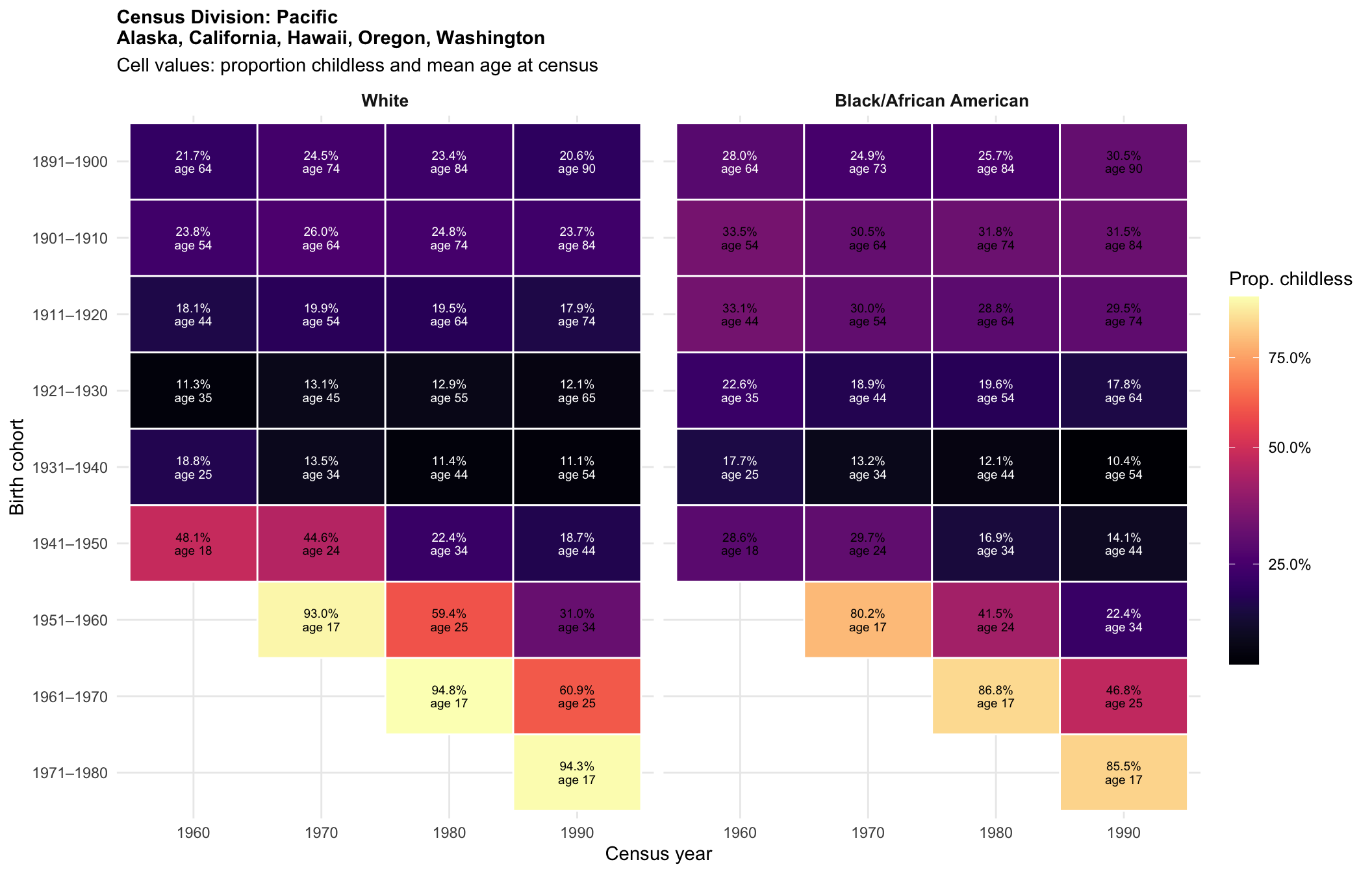
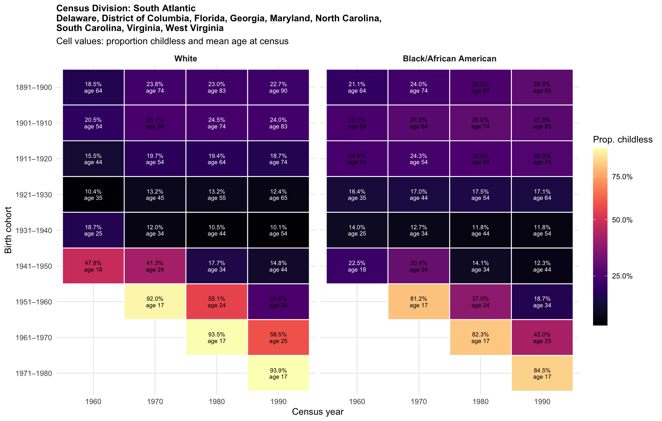
We track the proportion childless for birth cohorts as they age across census waves. Each cohort × age combination maps to exactly one census year, shown in all panels. Because CHBORN is completed-fertility-equivalent only at 50+, we exclude the 40–49 age group.

Observable cohort matrix (age at each census year):

Cohort	1960	1970	1980	1990
1891–1900	60–69	70–79	80–89	—
1901–1910	50–59	60–69	70–79	80–89
1911–1920	40–49	50–59	60–69	70–79
1921–1930	30–39	40–49	50–59	60–69
1931–1940	20–29	30–39	40–49	50–59
1941–1950	—	20–29	30–39	40–49
1951–1960	—	—	20–29	30–39
1961–1970	—	—	—	20–29

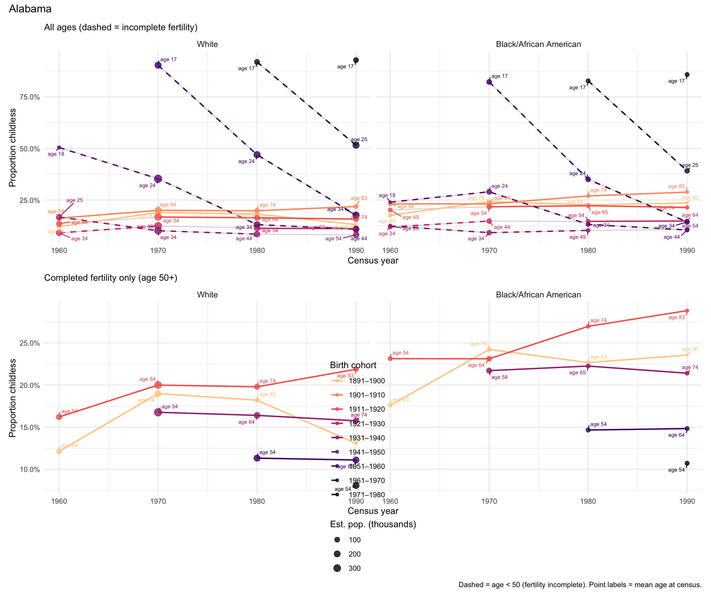
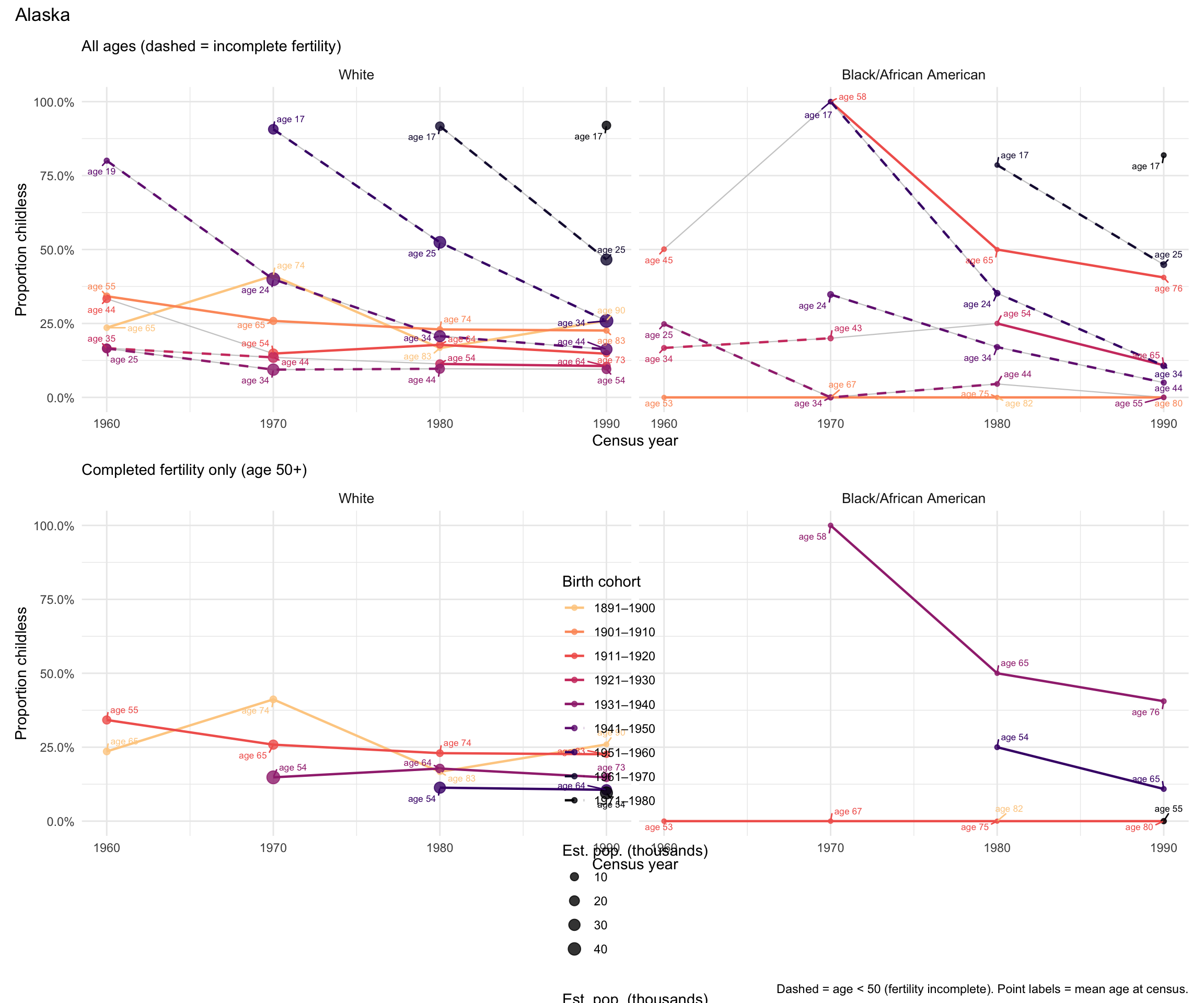
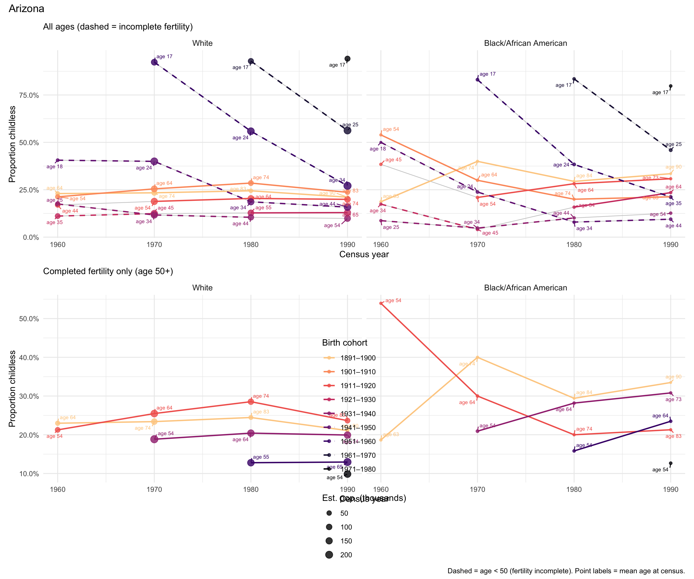
Bold = first completed-fertility observation (50+). Dashed lines in plots = incomplete fertility.

Survivorship bias: prop_zero may appear to rise as a cohort ages because women with children may have different mortality than childless women. Treat increases at ages 70–89 with caution.

data_cohort <- data_raw %>%
  prepare_cohort_sample() %>%
  mutate(state_name = as.character(STATEFIP))

# Cohorts observable in our 1960-1990 data across all age groups:
# Older cohorts (50+ completed fertility) + younger cohorts (20s-40s, incomplete)
cohorts_of_interest <- c(
  "1891–1900", "1901–1910", "1911–1920", "1921–1930",
  "1931–1940", "1941–1950", "1951–1960", "1961–1970",
  "1971–1980"
)

cat("Cohort data dimensions:", nrow(data_cohort), "rows\n")

Cohort data dimensions: 10740215 rows

cat("Age ranges:", levels(droplevels(data_cohort$AGE_RANGE)), "\n")

Age ranges: 15-19 20-29 30-39 40-49 50-59 60-69 70-79 80-89 

cat("Cohorts:", levels(droplevels(data_cohort$cohort_label)), "\n")

Cohorts: 1851–1860 1861–1870 1871–1880 1881–1890 1891–1900 1901–1910 1911–1920 1921–1930 1931–1940 1941–1950 1951–1960 1961–1970 1971–1980 

9a. National cohort trajectories

cohort_national <- data_cohort %>%
  group_by(cohort_label, YEAR, AGE_RANGE, RACE) %>%
  summarise(
    n_obs     = n(),
    prop_zero = weighted.mean(chborn_num == 0, w = PERWT),
    n_pop     = sum(PERWT),
    mean_age  = weighted.mean(AGE, w = PERWT),
    .groups   = "drop"
  ) %>%
  mutate(
    prop_zero = prop_zero,
    age_label = paste0("age ", round(mean_age)),
    completed = AGE_RANGE >= "50-59"
  ) %>%
  filter(cohort_label %in% cohorts_of_interest)

# Reusable two-panel cohort stability plot:
# Left = all ages combined; Right = completed fertility (50+) only
plot_cohort_stability <- function(df, title, pop_unit = 1e6, pop_label = "millions") {
  make_panel <- function(d, subtitle) {
    ggplot(d, aes(x = YEAR, y = prop_zero, color = cohort_label, group = cohort_label)) +
      geom_line(color = "grey80", linewidth = 0.4) +
      geom_line(data = subset(d,  completed), linewidth = 0.8) +
      geom_line(data = subset(d, !completed), linewidth = 0.8, linetype = "dashed") +
      geom_point(aes(size = n_pop / pop_unit), alpha = 0.8) +
      geom_text_repel(aes(label = age_label), size = 2.3, show.legend = FALSE,
                      min.segment.length = 0, box.padding = 0.3, seed = 42) +
      scale_x_continuous(breaks = c(1960, 1970, 1980, 1990)) +
      scale_y_continuous(labels = percent_format(accuracy = 0.1)) +
      scale_size_continuous(name = paste0("Est. pop. (", pop_label, ")"), range = c(1, 4)) +
      scale_color_viridis_d(option = "magma", direction = -1, end = 0.9, name = "Birth cohort") +
      facet_wrap(~ RACE) +
      labs(subtitle = subtitle,
           x = "Census year", y = "Proportion childless") +
      theme_minimal() +
      theme(strip.text = element_text(size = 10))
  }

  p_all  <- make_panel(df, "All ages (dashed = incomplete fertility)")
  p_comp <- make_panel(subset(df, completed), "Completed fertility only (age 50+)")

  (p_all / p_comp / guide_area()) +
    plot_layout(guides = "collect", heights = c(1, 1, 0.25)) +
    plot_annotation(
      title   = title,
      caption = "Dashed = age < 50 (fertility incomplete). Point labels = mean age at census."
    )
}

plot_cohort_stability(
  cohort_national %>% filter(!is.na(prop_zero)),
  title    = "Proportion Childless by Birth Cohort Across Census Years\nNon-Hispanic women, IPUMS USA 1960–1990",
  pop_unit  = 1e6,
  pop_label = "millions"
)

Past versions of cohort-national-plot-1.png

Version	Author	Date
5634d2b	Tina Lasisi	2026-04-16
027da76	Tina Lasisi	2026-04-14
71cf78a	Tina Lasisi	2026-04-14
34bd822	Tina Lasisi	2026-04-14
9d44b29	Tina Lasisi	2026-04-14
79eb4de	Tina Lasisi	2026-04-14

# All cohorts included in heatmap (not filtered to cohorts_of_interest)
data_cohort %>%
  group_by(cohort_label, YEAR, AGE_RANGE, RACE) %>%
  summarise(
    n_obs     = n(),
    prop_zero = weighted.mean(chborn_num == 0, w = PERWT),
    mean_age  = weighted.mean(AGE, w = PERWT),
    .groups   = "drop"
  ) %>%
  mutate(
    prop_zero = prop_zero,
    age_label = paste0("age ", round(mean_age))
  ) %>%
  mutate(
    cell_label  = if_else(
      !is.na(prop_zero),
      paste0(percent(prop_zero, accuracy = 0.1), "\n", age_label),
      "—"
    ),
    text_color = if_else(
      is.na(prop_zero) |
        prop_zero > quantile(prop_zero, 0.6, na.rm = TRUE),
      "black", "white"
    )
  ) %>%
  ggplot(aes(x = as.factor(YEAR), y = fct_rev(cohort_label), fill = prop_zero)) +
  geom_tile(color = "white", linewidth = 0.5) +
  geom_text(aes(label = cell_label, color = text_color), size = 2.8, lineheight = 0.9) +
  scale_color_identity() +
  scale_fill_viridis(
    option = "magma", na.value = "grey90",
    labels = percent_format(accuracy = 0.1),
    name   = "Prop. childless",
    trans  = "sqrt"
  ) +
  facet_wrap(~ RACE) +
  labs(
    title    = "Proportion Childless: Cohort × Census Year Matrix",
    subtitle = "Cell values show proportion and mean age of cohort at that census",
    x        = "Census year",
    y        = "Birth cohort"
  ) +
  theme_minimal() +
  theme(strip.text = element_text(size = 11, face = "bold"),
        legend.position = "right",
        legend.key.height = unit(1.5, "cm"))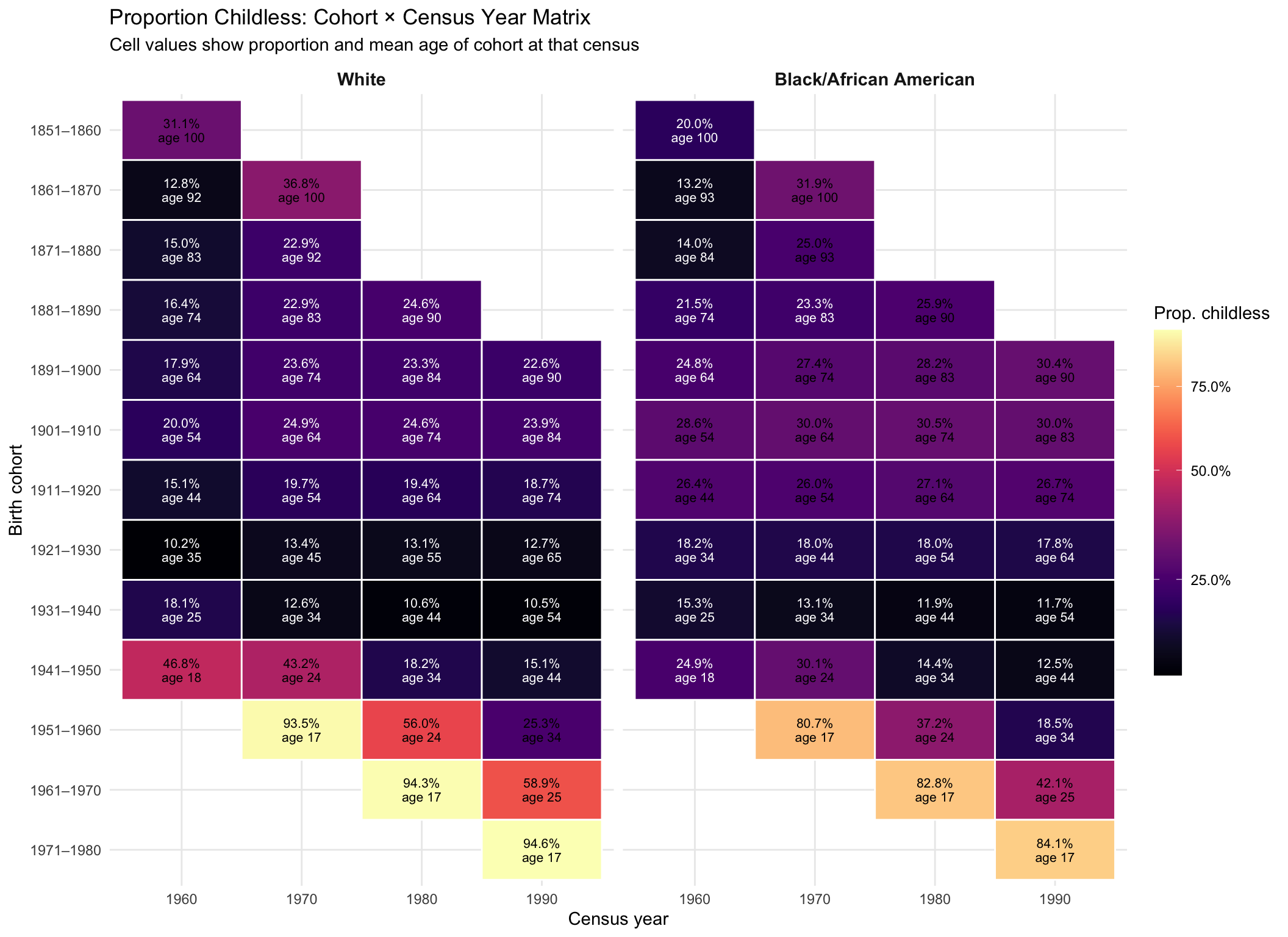

Past versions of cohort-national-heatmap-1.png

Version	Author	Date
5634d2b	Tina Lasisi	2026-04-16
71cf78a	Tina Lasisi	2026-04-14
34bd822	Tina Lasisi	2026-04-14
9d44b29	Tina Lasisi	2026-04-14
79eb4de	Tina Lasisi	2026-04-14

9b. State-level cohort analysis

For state-level analysis we require n ≥ 30 per cohort × age × race × state cell.

cohort_state <- data_cohort %>%
  group_by(state_name, cohort_label, YEAR, AGE_RANGE, RACE) %>%
  summarise(
    n_obs     = n(),
    prop_zero = weighted.mean(chborn_num == 0, w = PERWT),
    n_pop     = sum(PERWT),
    mean_age  = weighted.mean(AGE, w = PERWT),
    .groups   = "drop"
  ) %>%
  mutate(
    prop_zero = prop_zero,
    age_label = paste0("age ", round(mean_age)),
    completed = AGE_RANGE >= "50-59"
  ) %>%
  filter(cohort_label %in% cohorts_of_interest)

Choropleth maps: Birth Cohort × Age Group

# Grid: rows = birth cohort, columns = census year
# Panel title shows the age group that cohort was at that census year
# Shared colour scale across all panels for direct comparison

plot_cohort_grid <- function(df, race_filter, palette_option = "magma") {
  df <- df %>%
    filter(RACE == race_filter) %>%
    rename(state = state_name)

  lims    <- range(df$prop_zero, na.rm = TRUE)
  cohorts <- sort(unique(df$cohort_label))
  ages    <- levels(df$AGE_RANGE)  # ordered factor: 15-19 ... 80-89

  plots <- list()
  for (ag in ages) {
    for (ch in cohorts) {
      sub <- df %>% filter(AGE_RANGE == ag, cohort_label == ch)
      # derive census year for subtitle
      yr_lab <- if (nrow(sub) > 0) paste(sort(unique(sub$YEAR)), collapse = "/") else "—"
      panel_title <- paste0(ch, "\n", ag, "\n(", yr_lab, ")")

      if (nrow(sub) > 0 && any(!is.na(sub$prop_zero))) {
        p <- plot_usmap(data = sub, values = "prop_zero",
                        color = "grey70", linewidth = 0.15) +
          scale_fill_viridis(option = palette_option, na.value = "grey90",
                             name = NULL, limits = lims, trans = "sqrt") +
          labs(title = panel_title) +
          theme(plot.title = element_text(size = 6.5, hjust = 0.5))
      } else {
        p <- ggplot() + theme_void() +
          labs(title = panel_title) +
          theme(plot.title = element_text(size = 6.5, hjust = 0.5, color = "grey60"))
      }
      plots <- c(plots, list(p))
    }
  }

  # columns = cohorts, rows = age groups
  wrap_plots(plots, ncol = length(cohorts)) +
    plot_layout(guides = "collect") +
    plot_annotation(
      title    = paste0("Proportion Childless: Birth Cohort × Age Group\n", race_filter),
      subtitle = "Rows = age group  |  Columns = birth cohort  |  Panel label shows cohort, age group, census year",
      caption  = "Proportion reporting zero children ever born (CHBORN = 0), weighted by PERWT. Shared colour scale. Source: IPUMS USA 1% samples."
    ) &
    theme(legend.position = "right",
          plot.title = element_text(size = 13, hjust = 0.5))
}

plot_cohort_grid(cohort_state, "White")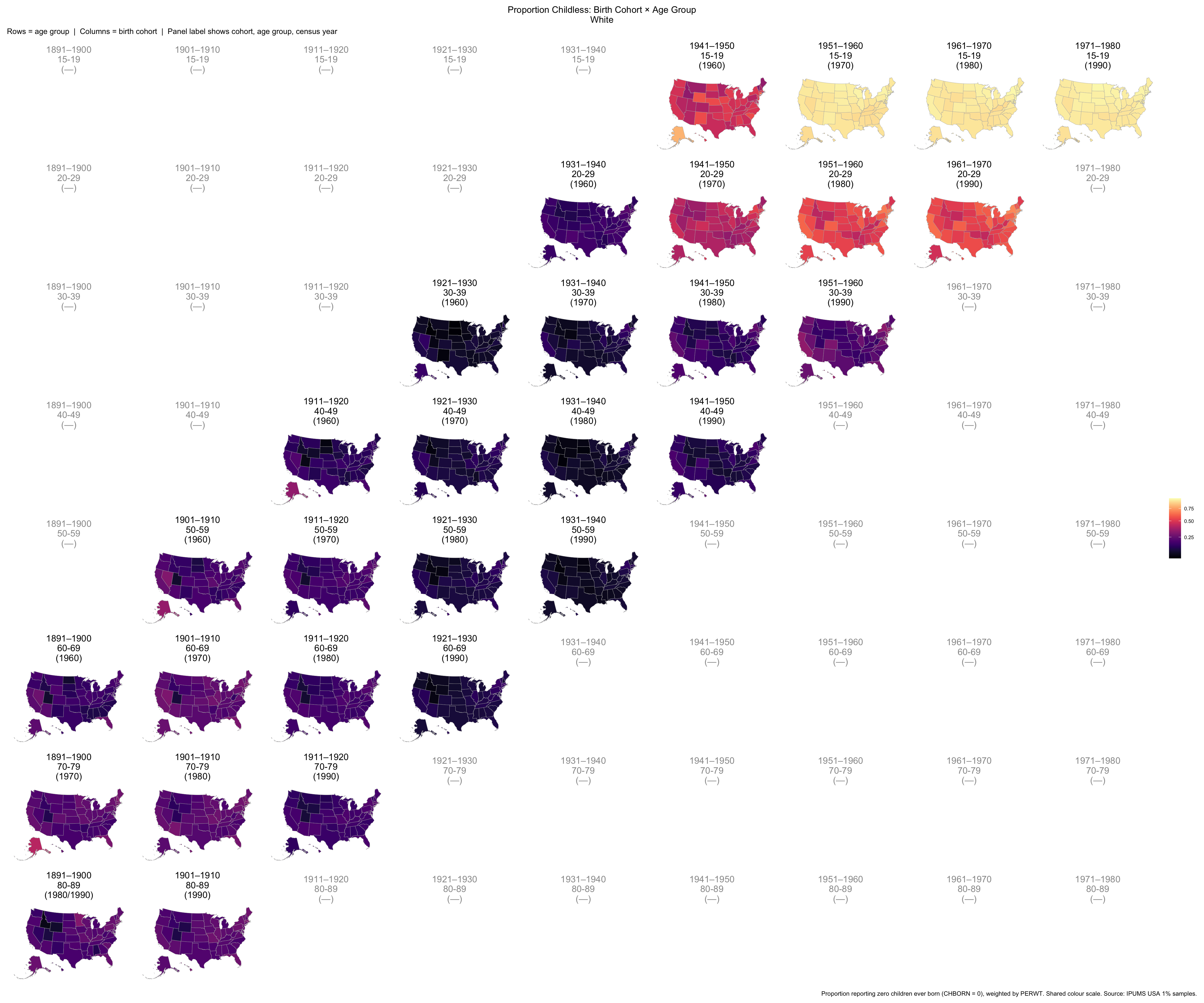

Past versions of cohort-state-maps-1.png

Version	Author	Date
5634d2b	Tina Lasisi	2026-04-16
71cf78a	Tina Lasisi	2026-04-14
34bd822	Tina Lasisi	2026-04-14
9d44b29	Tina Lasisi	2026-04-14
79eb4de	Tina Lasisi	2026-04-14

plot_cohort_grid(cohort_state, "Black/African American")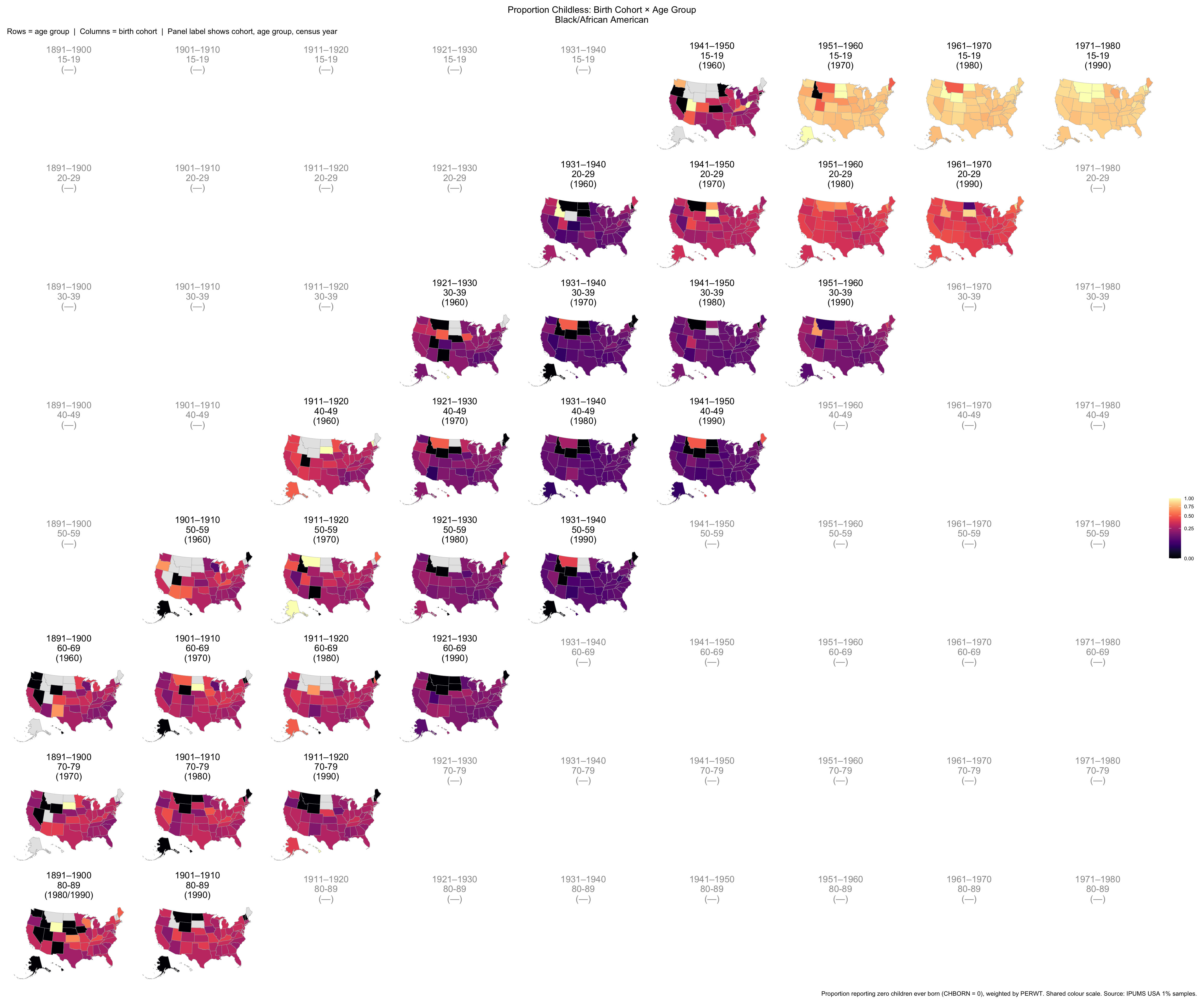

Past versions of cohort-state-maps-black-1.png

Version	Author	Date
5634d2b	Tina Lasisi	2026-04-16
71cf78a	Tina Lasisi	2026-04-14
34bd822	Tina Lasisi	2026-04-14
9d44b29	Tina Lasisi	2026-04-14
79eb4de	Tina Lasisi	2026-04-14

# Regional choropleth grid: each state is coloured by its region's prop_zero.
# regional_df  : summarised data with columns (group_var, cohort_label, YEAR,
#                AGE_RANGE, RACE, prop_zero)
# group_var    : name of the grouping column ("division" or "conference")
# state_lookup : function(state_name) -> group label (state_to_division / state_to_conference)
# all_states   : character vector of all state names in the data
plot_cohort_grid_regional <- function(regional_df, race_filter,
                                      group_var, state_lookup,
                                      all_states,
                                      palette_option = "magma") {
  df <- regional_df %>% filter(RACE == race_filter)

  lims    <- range(df$prop_zero, na.rm = TRUE)
  cohorts <- sort(unique(df$cohort_label))
  ages    <- levels(df$AGE_RANGE)

  # Build a state-level lookup table: state -> group label
  state_group <- tibble(
    state = all_states,
    grp   = state_lookup(all_states)
  ) %>% filter(!is.na(grp))

  plots <- list()
  for (ag in ages) {
    for (ch in cohorts) {
      sub_reg <- df %>% filter(AGE_RANGE == ag, cohort_label == ch)
      yr_lab  <- if (nrow(sub_reg) > 0) paste(sort(unique(sub_reg$YEAR)), collapse = "/") else "—"
      panel_title <- paste0(ch, "\n", ag, "\n(", yr_lab, ")")

      if (nrow(sub_reg) > 0 && any(!is.na(sub_reg$prop_zero))) {
        # Join regional values onto each state
        sub_state <- state_group %>%
          left_join(
            sub_reg %>% select(grp = all_of(group_var), prop_zero),
            by = "grp"
          )

        p <- plot_usmap(data = sub_state, values = "prop_zero",
                        color = "grey70", linewidth = 0.15) +
          scale_fill_viridis(option = palette_option, na.value = "grey90",
                             name = NULL, limits = lims, trans = "sqrt") +
          labs(title = panel_title) +
          theme(plot.title = element_text(size = 6.5, hjust = 0.5))
      } else {
        p <- ggplot() + theme_void() +
          labs(title = panel_title) +
          theme(plot.title = element_text(size = 6.5, hjust = 0.5, color = "grey60"))
      }
      plots <- c(plots, list(p))
    }
  }

  wrap_plots(plots, ncol = length(cohorts)) +
    plot_layout(guides = "collect") +
    plot_annotation(
      title    = paste0("Proportion Childless: Birth Cohort × Age Group\n",
                        race_filter, " — by ", group_var),
      subtitle = "Rows = age group  |  Columns = birth cohort  |  States coloured by regional value",
      caption  = "Proportion reporting zero children ever born (CHBORN = 0), weighted by PERWT. Source: IPUMS USA 1% samples."
    ) &
    theme(legend.position = "right",
          plot.title = element_text(size = 13, hjust = 0.5))
}

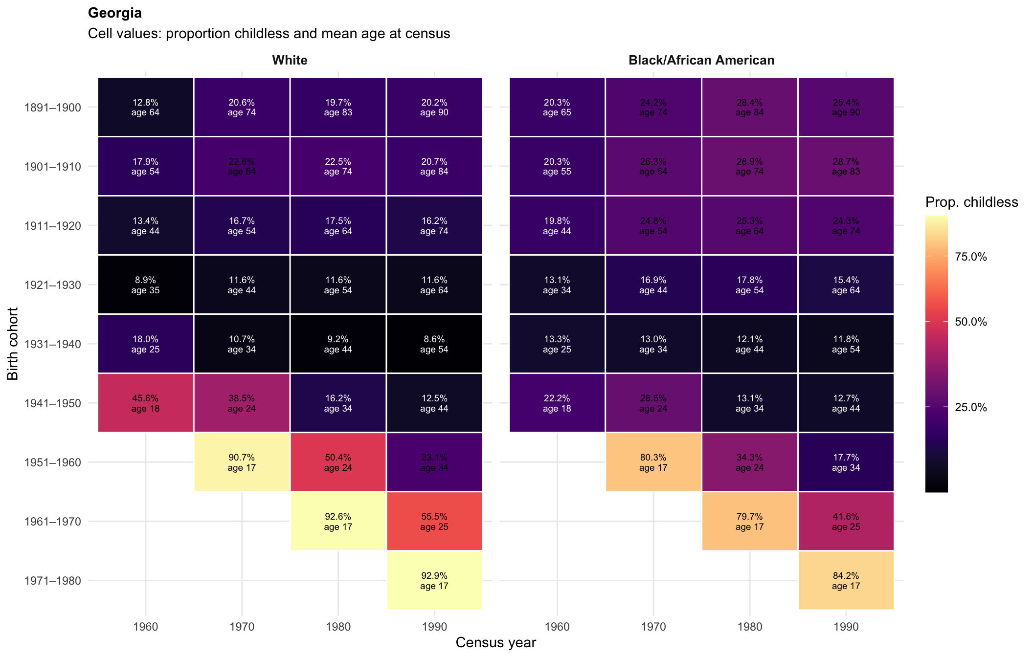
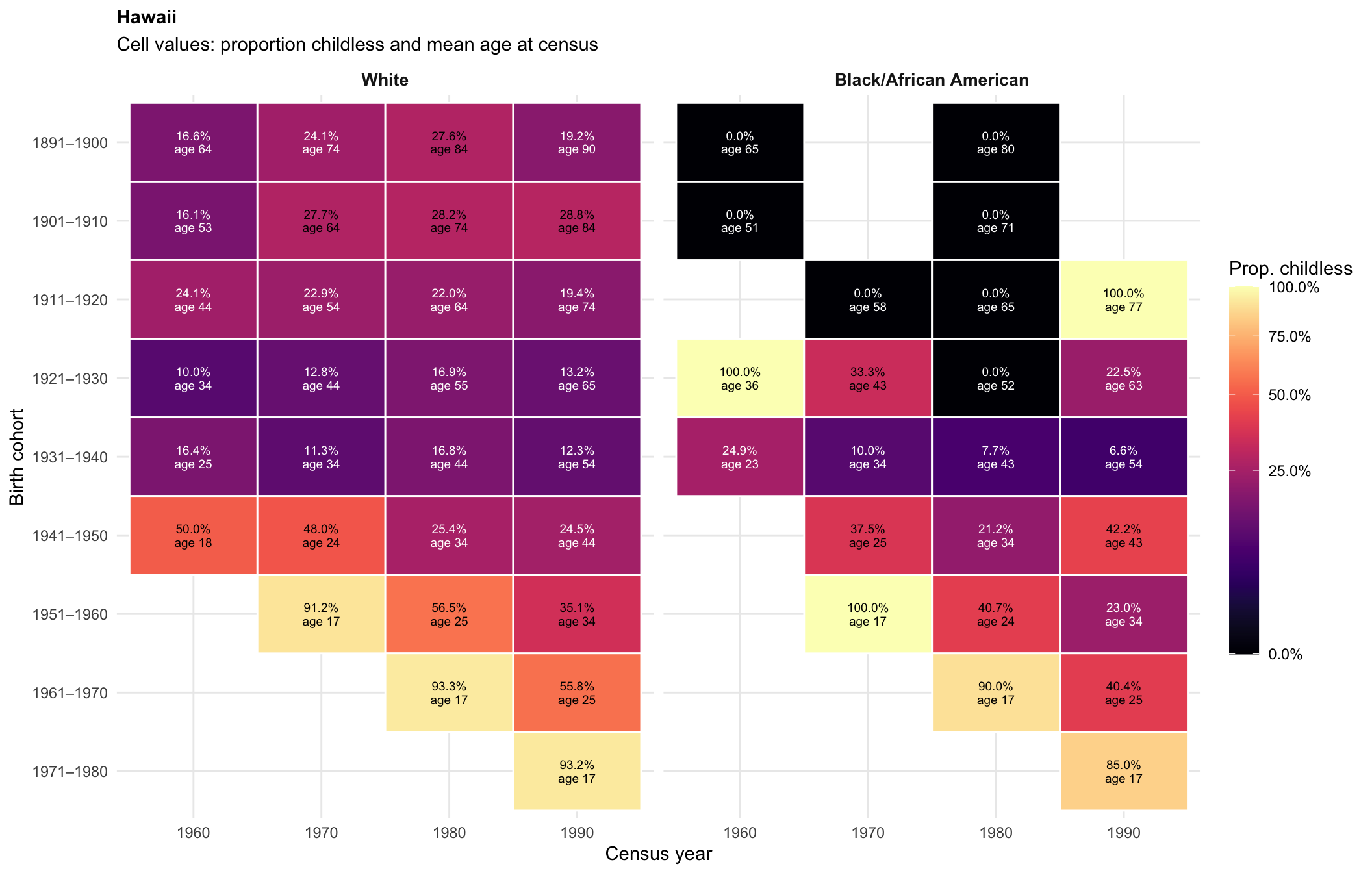
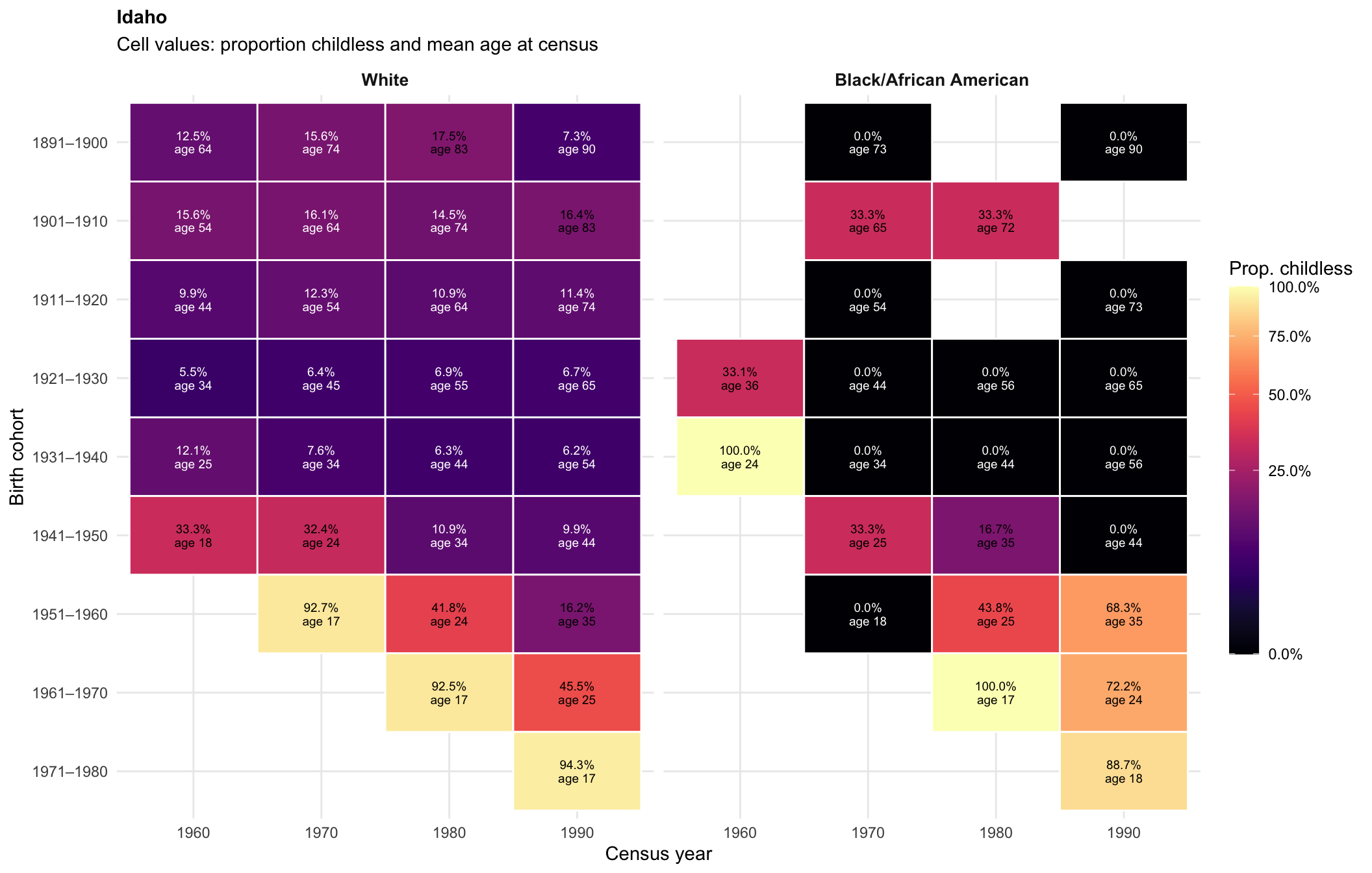
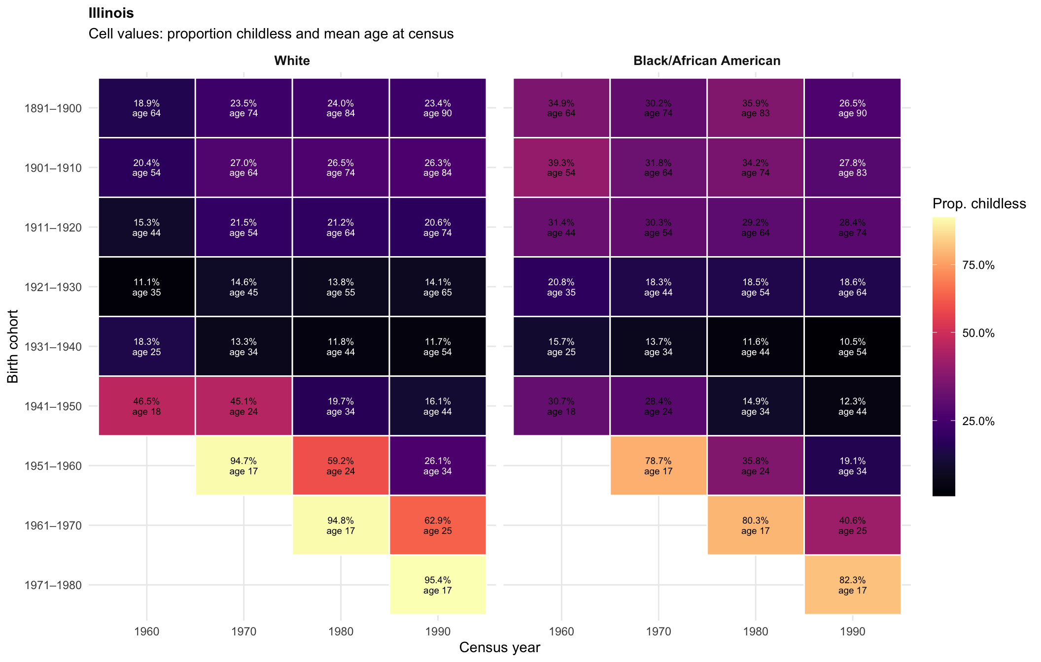
Cohort × Census Year matrices (per state)

# Reusable cohort × census year heatmap for a single grouping unit (state, division, etc.)
plot_cohort_matrix <- function(df, title) {
  df %>%
    mutate(
      cell_label = if_else(
        !is.na(prop_zero),
        paste0(percent(prop_zero, accuracy = 0.1), "\n", age_label),
        "—"
      ),
      text_color = if_else(
        is.na(prop_zero) |
          prop_zero > quantile(prop_zero, 0.6, na.rm = TRUE),
        "black", "white"
      )
    ) %>%
    ggplot(aes(x = as.factor(YEAR), y = fct_rev(cohort_label), fill = prop_zero)) +
    geom_tile(color = "white", linewidth = 0.5) +
    geom_text(aes(label = cell_label, color = text_color), size = 2.5, lineheight = 0.9) +
    scale_color_identity() +
    scale_fill_viridis(
      option = "magma", na.value = "grey90",
      labels = percent_format(accuracy = 0.1),
      name   = "Prop. childless",
      trans  = "sqrt"
    ) +
    facet_wrap(~ RACE) +
    labs(
      title    = title,
      subtitle = "Cell values: proportion childless and mean age at census",
      x        = "Census year",
      y        = "Birth cohort"
    ) +
    theme_minimal() +
    theme(strip.text = element_text(size = 10, face = "bold"),
          plot.title = element_text(size = 11, face = "bold"),
          legend.position = "right",
          legend.key.height = unit(1.5, "cm"))
}

all_states <- sort(unique(cohort_state$state_name))

for (st in all_states) {
  st_mat <- cohort_state %>%
    filter(state_name == st)

  if (nrow(st_mat) == 0) next

  p <- plot_cohort_matrix(st_mat, title = st)
  print(p)
  cat("\n\n")
}

Past versions of cohort-state-matrix-1.png

Version	Author	Date
5634d2b	Tina Lasisi	2026-04-16

Past versions of cohort-state-matrix-2.png

Version	Author	Date
5634d2b	Tina Lasisi	2026-04-16

Past versions of cohort-state-matrix-3.png

Version	Author	Date
5634d2b	Tina Lasisi	2026-04-16

Past versions of cohort-state-matrix-4.png

Version	Author	Date
5634d2b	Tina Lasisi	2026-04-16

Past versions of cohort-state-matrix-5.png

Version	Author	Date
5634d2b	Tina Lasisi	2026-04-16

Past versions of cohort-state-matrix-6.png

Version	Author	Date
5634d2b	Tina Lasisi	2026-04-16

Past versions of cohort-state-matrix-7.png

Version	Author	Date
5634d2b	Tina Lasisi	2026-04-16

Past versions of cohort-state-matrix-8.png

Version	Author	Date
5634d2b	Tina Lasisi	2026-04-16

Past versions of cohort-state-matrix-9.png

Version	Author	Date
5634d2b	Tina Lasisi	2026-04-16

Past versions of cohort-state-matrix-10.png

Version	Author	Date
5634d2b	Tina Lasisi	2026-04-16

Past versions of cohort-state-matrix-11.png

Version	Author	Date
5634d2b	Tina Lasisi	2026-04-16

Past versions of cohort-state-matrix-12.png

Version	Author	Date
5634d2b	Tina Lasisi	2026-04-16

Past versions of cohort-state-matrix-13.png

Version	Author	Date
5634d2b	Tina Lasisi	2026-04-16

Past versions of cohort-state-matrix-14.png

Version	Author	Date
5634d2b	Tina Lasisi	2026-04-16

Past versions of cohort-state-matrix-15.png

Version	Author	Date
5634d2b	Tina Lasisi	2026-04-16

Past versions of cohort-state-matrix-16.png

Version	Author	Date
5634d2b	Tina Lasisi	2026-04-16

Past versions of cohort-state-matrix-17.png

Version	Author	Date
5634d2b	Tina Lasisi	2026-04-16

Past versions of cohort-state-matrix-18.png

Version	Author	Date
5634d2b	Tina Lasisi	2026-04-16

Past versions of cohort-state-matrix-19.png

Version	Author	Date
5634d2b	Tina Lasisi	2026-04-16

Past versions of cohort-state-matrix-20.png

Version	Author	Date
5634d2b	Tina Lasisi	2026-04-16

Past versions of cohort-state-matrix-21.png

Version	Author	Date
5634d2b	Tina Lasisi	2026-04-16

Past versions of cohort-state-matrix-22.png

Version	Author	Date
5634d2b	Tina Lasisi	2026-04-16

Past versions of cohort-state-matrix-23.png

Version	Author	Date
5634d2b	Tina Lasisi	2026-04-16

Past versions of cohort-state-matrix-24.png

Version	Author	Date
5634d2b	Tina Lasisi	2026-04-16

Past versions of cohort-state-matrix-25.png

Version	Author	Date
5634d2b	Tina Lasisi	2026-04-16

Past versions of cohort-state-matrix-26.png

Version	Author	Date
5634d2b	Tina Lasisi	2026-04-16

Past versions of cohort-state-matrix-27.png

Version	Author	Date
5634d2b	Tina Lasisi	2026-04-16

Past versions of cohort-state-matrix-28.png

Version	Author	Date
5634d2b	Tina Lasisi	2026-04-16

Past versions of cohort-state-matrix-29.png

Version	Author	Date
5634d2b	Tina Lasisi	2026-04-16

Past versions of cohort-state-matrix-30.png

Version	Author	Date
5634d2b	Tina Lasisi	2026-04-16

Past versions of cohort-state-matrix-31.png

Version	Author	Date
5634d2b	Tina Lasisi	2026-04-16

Past versions of cohort-state-matrix-32.png

Version	Author	Date
5634d2b	Tina Lasisi	2026-04-16

Past versions of cohort-state-matrix-33.png

Version	Author	Date
5634d2b	Tina Lasisi	2026-04-16

Past versions of cohort-state-matrix-34.png

Version	Author	Date
5634d2b	Tina Lasisi	2026-04-16

Past versions of cohort-state-matrix-35.png

Version	Author	Date
5634d2b	Tina Lasisi	2026-04-16

Past versions of cohort-state-matrix-36.png

Version	Author	Date
5634d2b	Tina Lasisi	2026-04-16

Past versions of cohort-state-matrix-37.png

Version	Author	Date
5634d2b	Tina Lasisi	2026-04-16

Past versions of cohort-state-matrix-38.png

Version	Author	Date
5634d2b	Tina Lasisi	2026-04-16

Past versions of cohort-state-matrix-39.png

Version	Author	Date
5634d2b	Tina Lasisi	2026-04-16

Past versions of cohort-state-matrix-40.png

Version	Author	Date
5634d2b	Tina Lasisi	2026-04-16

Past versions of cohort-state-matrix-41.png

Version	Author	Date
5634d2b	Tina Lasisi	2026-04-16

Past versions of cohort-state-matrix-42.png

Version	Author	Date
5634d2b	Tina Lasisi	2026-04-16

Past versions of cohort-state-matrix-43.png

Version	Author	Date
5634d2b	Tina Lasisi	2026-04-16

Past versions of cohort-state-matrix-44.png

Version	Author	Date
5634d2b	Tina Lasisi	2026-04-16

Past versions of cohort-state-matrix-45.png

Version	Author	Date
5634d2b	Tina Lasisi	2026-04-16

Past versions of cohort-state-matrix-46.png

Version	Author	Date
5634d2b	Tina Lasisi	2026-04-16

Past versions of cohort-state-matrix-47.png

Version	Author	Date
5634d2b	Tina Lasisi	2026-04-16

Past versions of cohort-state-matrix-48.png

Version	Author	Date
5634d2b	Tina Lasisi	2026-04-16

Past versions of cohort-state-matrix-49.png

Version	Author	Date
5634d2b	Tina Lasisi	2026-04-16

Past versions of cohort-state-matrix-50.png

Version	Author	Date
5634d2b	Tina Lasisi	2026-04-16

Past versions of cohort-state-matrix-51.png

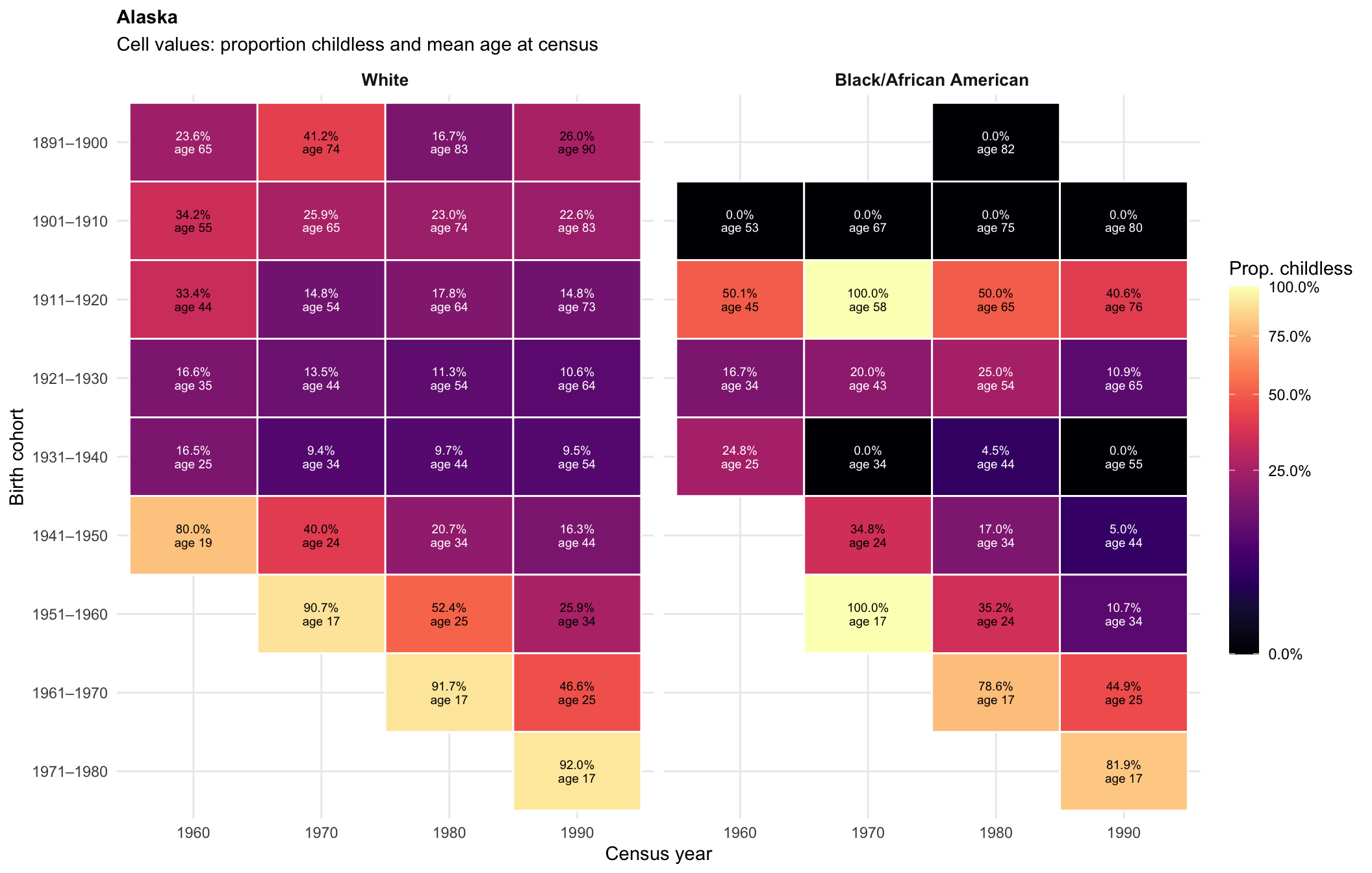
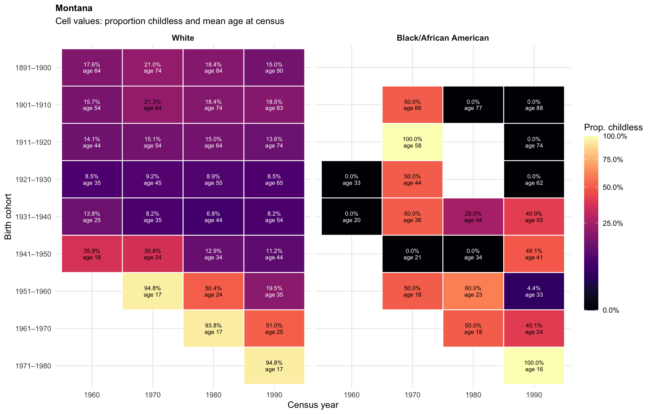
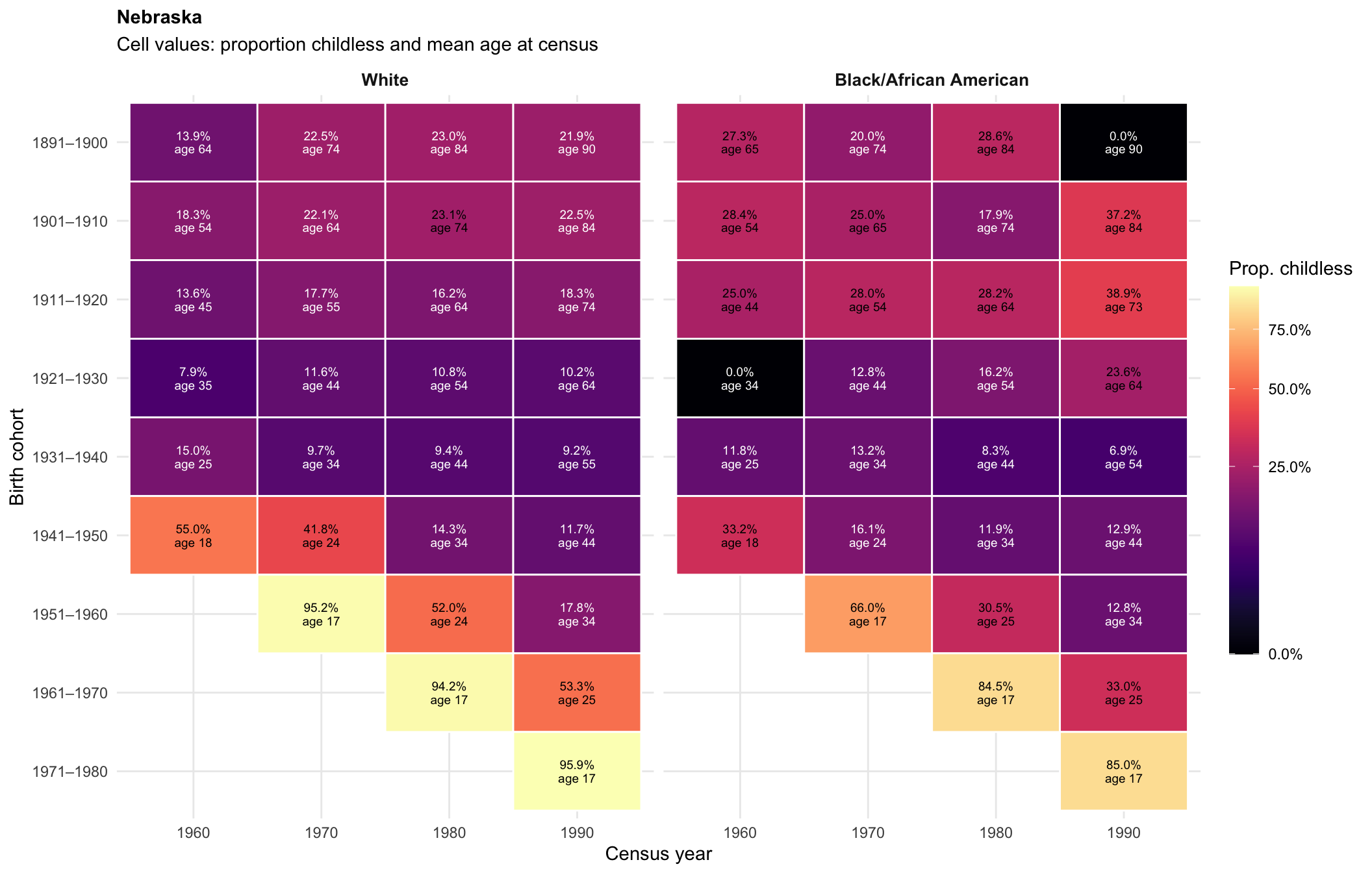
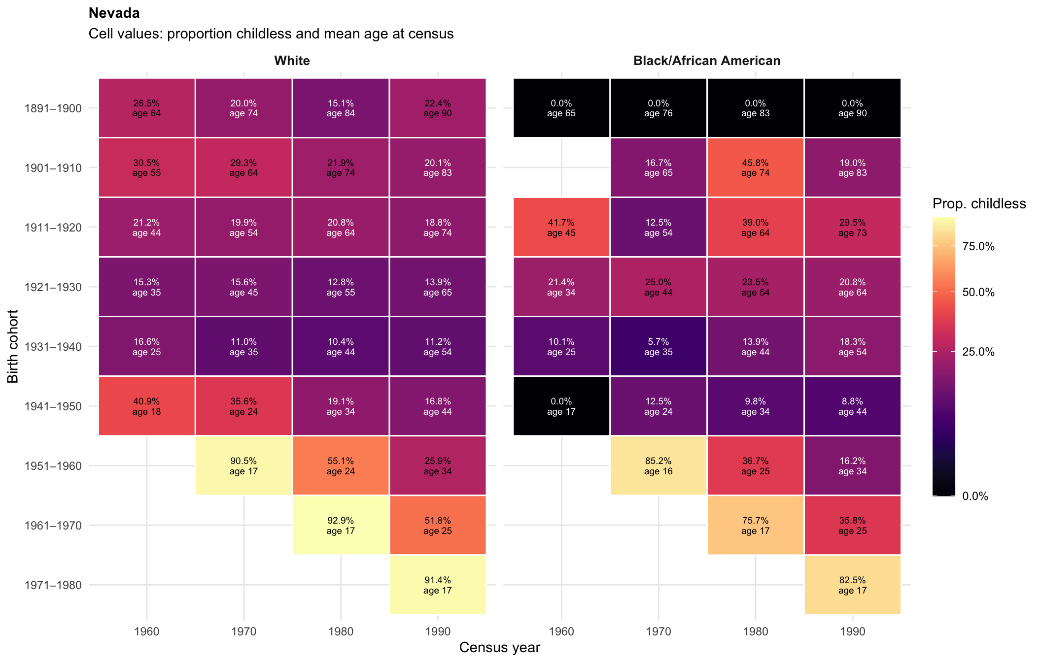
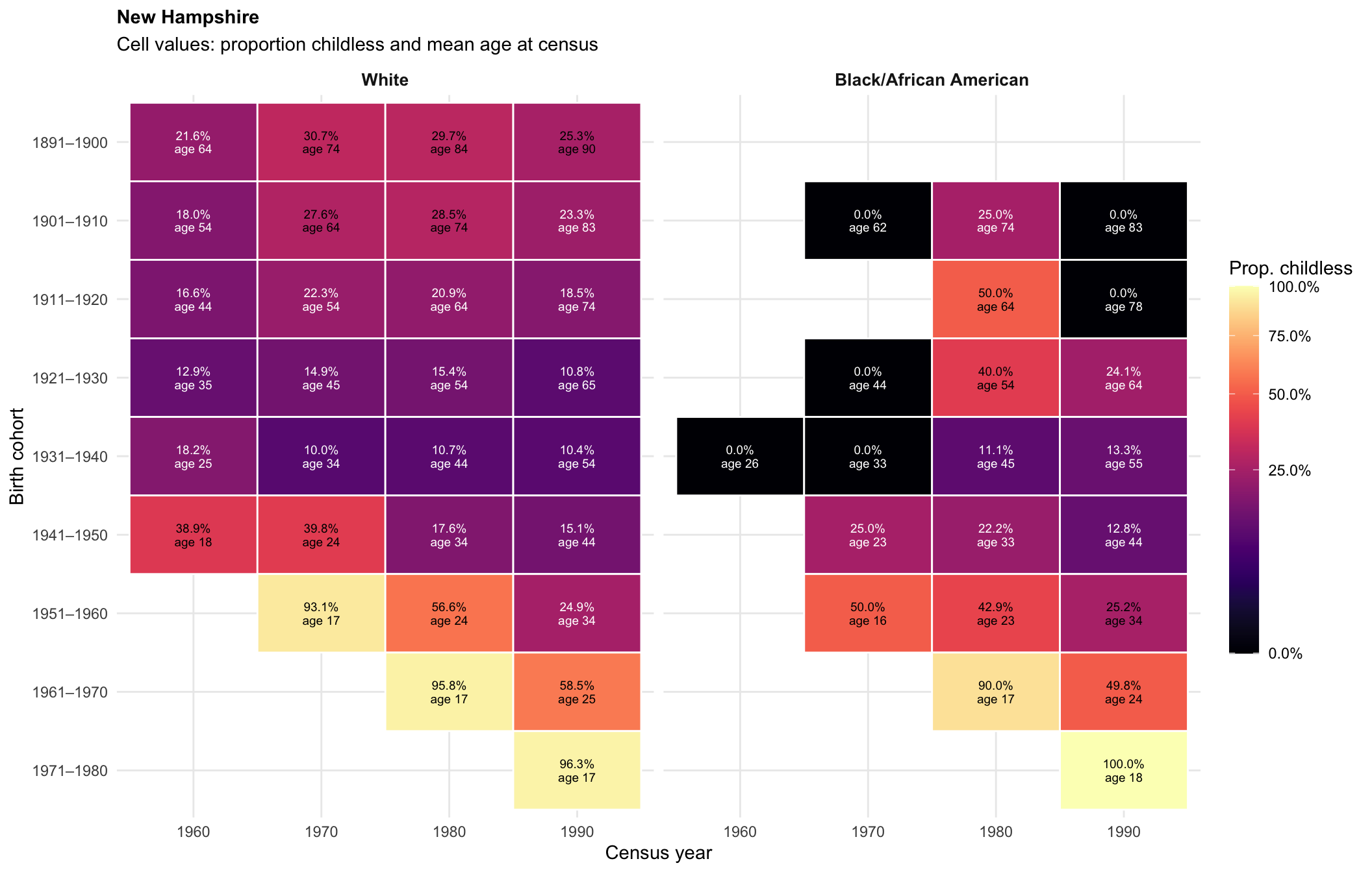
Version	Author	Date
5634d2b	Tina Lasisi	2026-04-16

Trajectory plots (per state)

eligible_cohort_states <- cohort_state %>%
  filter(!is.na(prop_zero)) %>%
  group_by(state_name, RACE) %>%
  summarise(n_points = n_distinct(paste(cohort_label, YEAR)), .groups = "drop") %>%
  filter(n_points >= 2) %>%
  pull(state_name) %>%
  unique() %>%
  sort()

cat(length(eligible_cohort_states),
    "states with adequate cohort data for trajectory plots\n")

51 states with adequate cohort data for trajectory plots

for (st in eligible_cohort_states) {
  st_cohort <- cohort_state %>%
    filter(state_name == st, !is.na(prop_zero))

  if (nrow(st_cohort) == 0) next

  p <- plot_cohort_stability(st_cohort, title = st,
                             pop_unit = 1e3, pop_label = "thousands")

  print(p)
  cat("\n\n")
}

Past versions of cohort-state-trajectories-1.png

Version	Author	Date
5634d2b	Tina Lasisi	2026-04-16
027da76	Tina Lasisi	2026-04-14
71cf78a	Tina Lasisi	2026-04-14
34bd822	Tina Lasisi	2026-04-14
9d44b29	Tina Lasisi	2026-04-14
79eb4de	Tina Lasisi	2026-04-14

Past versions of cohort-state-trajectories-2.png

Version	Author	Date
5634d2b	Tina Lasisi	2026-04-16
027da76	Tina Lasisi	2026-04-14
71cf78a	Tina Lasisi	2026-04-14
34bd822	Tina Lasisi	2026-04-14
9d44b29	Tina Lasisi	2026-04-14
79eb4de	Tina Lasisi	2026-04-14

Past versions of cohort-state-trajectories-3.png

Version	Author	Date
5634d2b	Tina Lasisi	2026-04-16
027da76	Tina Lasisi	2026-04-14
71cf78a	Tina Lasisi	2026-04-14
34bd822	Tina Lasisi	2026-04-14
9d44b29	Tina Lasisi	2026-04-14
79eb4de	Tina Lasisi	2026-04-14

Past versions of cohort-state-trajectories-4.png

Version	Author	Date
5634d2b	Tina Lasisi	2026-04-16
027da76	Tina Lasisi	2026-04-14
71cf78a	Tina Lasisi	2026-04-14
34bd822	Tina Lasisi	2026-04-14
9d44b29	Tina Lasisi	2026-04-14
79eb4de	Tina Lasisi	2026-04-14

Past versions of cohort-state-trajectories-5.png

Version	Author	Date
5634d2b	Tina Lasisi	2026-04-16
027da76	Tina Lasisi	2026-04-14
71cf78a	Tina Lasisi	2026-04-14
34bd822	Tina Lasisi	2026-04-14
9d44b29	Tina Lasisi	2026-04-14
79eb4de	Tina Lasisi	2026-04-14

Past versions of cohort-state-trajectories-6.png

Version	Author	Date
5634d2b	Tina Lasisi	2026-04-16
027da76	Tina Lasisi	2026-04-14
71cf78a	Tina Lasisi	2026-04-14
34bd822	Tina Lasisi	2026-04-14
9d44b29	Tina Lasisi	2026-04-14
79eb4de	Tina Lasisi	2026-04-14

Past versions of cohort-state-trajectories-7.png

Version	Author	Date
5634d2b	Tina Lasisi	2026-04-16
027da76	Tina Lasisi	2026-04-14
71cf78a	Tina Lasisi	2026-04-14
34bd822	Tina Lasisi	2026-04-14
9d44b29	Tina Lasisi	2026-04-14
79eb4de	Tina Lasisi	2026-04-14

Past versions of cohort-state-trajectories-8.png

Version	Author	Date
5634d2b	Tina Lasisi	2026-04-16
027da76	Tina Lasisi	2026-04-14
71cf78a	Tina Lasisi	2026-04-14
34bd822	Tina Lasisi	2026-04-14
9d44b29	Tina Lasisi	2026-04-14
79eb4de	Tina Lasisi	2026-04-14

Past versions of cohort-state-trajectories-9.png

Version	Author	Date
5634d2b	Tina Lasisi	2026-04-16
027da76	Tina Lasisi	2026-04-14
71cf78a	Tina Lasisi	2026-04-14
34bd822	Tina Lasisi	2026-04-14
9d44b29	Tina Lasisi	2026-04-14
79eb4de	Tina Lasisi	2026-04-14

Past versions of cohort-state-trajectories-10.png

Version	Author	Date
5634d2b	Tina Lasisi	2026-04-16
027da76	Tina Lasisi	2026-04-14
71cf78a	Tina Lasisi	2026-04-14
34bd822	Tina Lasisi	2026-04-14
9d44b29	Tina Lasisi	2026-04-14
79eb4de	Tina Lasisi	2026-04-14

Past versions of cohort-state-trajectories-11.png

Version	Author	Date
5634d2b	Tina Lasisi	2026-04-16
027da76	Tina Lasisi	2026-04-14
71cf78a	Tina Lasisi	2026-04-14
34bd822	Tina Lasisi	2026-04-14
9d44b29	Tina Lasisi	2026-04-14
79eb4de	Tina Lasisi	2026-04-14

Past versions of cohort-state-trajectories-12.png

Version	Author	Date
5634d2b	Tina Lasisi	2026-04-16
027da76	Tina Lasisi	2026-04-14
71cf78a	Tina Lasisi	2026-04-14
34bd822	Tina Lasisi	2026-04-14
9d44b29	Tina Lasisi	2026-04-14
79eb4de	Tina Lasisi	2026-04-14

Past versions of cohort-state-trajectories-13.png

Version	Author	Date
5634d2b	Tina Lasisi	2026-04-16
027da76	Tina Lasisi	2026-04-14
71cf78a	Tina Lasisi	2026-04-14
34bd822	Tina Lasisi	2026-04-14
9d44b29	Tina Lasisi	2026-04-14
79eb4de	Tina Lasisi	2026-04-14

Past versions of cohort-state-trajectories-14.png

Version	Author	Date
5634d2b	Tina Lasisi	2026-04-16
027da76	Tina Lasisi	2026-04-14
71cf78a	Tina Lasisi	2026-04-14
34bd822	Tina Lasisi	2026-04-14
9d44b29	Tina Lasisi	2026-04-14
79eb4de	Tina Lasisi	2026-04-14

Past versions of cohort-state-trajectories-15.png

Version	Author	Date
5634d2b	Tina Lasisi	2026-04-16
027da76	Tina Lasisi	2026-04-14
71cf78a	Tina Lasisi	2026-04-14
34bd822	Tina Lasisi	2026-04-14
9d44b29	Tina Lasisi	2026-04-14
79eb4de	Tina Lasisi	2026-04-14

Past versions of cohort-state-trajectories-16.png

Version	Author	Date
5634d2b	Tina Lasisi	2026-04-16
027da76	Tina Lasisi	2026-04-14
71cf78a	Tina Lasisi	2026-04-14
34bd822	Tina Lasisi	2026-04-14
9d44b29	Tina Lasisi	2026-04-14
79eb4de	Tina Lasisi	2026-04-14

Past versions of cohort-state-trajectories-17.png

Version	Author	Date
5634d2b	Tina Lasisi	2026-04-16
027da76	Tina Lasisi	2026-04-14
71cf78a	Tina Lasisi	2026-04-14
34bd822	Tina Lasisi	2026-04-14
9d44b29	Tina Lasisi	2026-04-14
79eb4de	Tina Lasisi	2026-04-14

Past versions of cohort-state-trajectories-18.png

Version	Author	Date
5634d2b	Tina Lasisi	2026-04-16
027da76	Tina Lasisi	2026-04-14
71cf78a	Tina Lasisi	2026-04-14
34bd822	Tina Lasisi	2026-04-14
9d44b29	Tina Lasisi	2026-04-14
79eb4de	Tina Lasisi	2026-04-14

Past versions of cohort-state-trajectories-19.png

Version	Author	Date
5634d2b	Tina Lasisi	2026-04-16
027da76	Tina Lasisi	2026-04-14
71cf78a	Tina Lasisi	2026-04-14
34bd822	Tina Lasisi	2026-04-14
9d44b29	Tina Lasisi	2026-04-14
79eb4de	Tina Lasisi	2026-04-14

Past versions of cohort-state-trajectories-20.png

Version	Author	Date
5634d2b	Tina Lasisi	2026-04-16
027da76	Tina Lasisi	2026-04-14
71cf78a	Tina Lasisi	2026-04-14
34bd822	Tina Lasisi	2026-04-14
9d44b29	Tina Lasisi	2026-04-14
79eb4de	Tina Lasisi	2026-04-14

Past versions of cohort-state-trajectories-21.png

Version	Author	Date
5634d2b	Tina Lasisi	2026-04-16
027da76	Tina Lasisi	2026-04-14
71cf78a	Tina Lasisi	2026-04-14
34bd822	Tina Lasisi	2026-04-14
9d44b29	Tina Lasisi	2026-04-14
79eb4de	Tina Lasisi	2026-04-14

Past versions of cohort-state-trajectories-22.png

Version	Author	Date
5634d2b	Tina Lasisi	2026-04-16
027da76	Tina Lasisi	2026-04-14
71cf78a	Tina Lasisi	2026-04-14
34bd822	Tina Lasisi	2026-04-14
9d44b29	Tina Lasisi	2026-04-14
79eb4de	Tina Lasisi	2026-04-14

Past versions of cohort-state-trajectories-23.png

Version	Author	Date
5634d2b	Tina Lasisi	2026-04-16
027da76	Tina Lasisi	2026-04-14
71cf78a	Tina Lasisi	2026-04-14
34bd822	Tina Lasisi	2026-04-14
9d44b29	Tina Lasisi	2026-04-14
79eb4de	Tina Lasisi	2026-04-14

Past versions of cohort-state-trajectories-24.png

Version	Author	Date
5634d2b	Tina Lasisi	2026-04-16
027da76	Tina Lasisi	2026-04-14
71cf78a	Tina Lasisi	2026-04-14
34bd822	Tina Lasisi	2026-04-14
9d44b29	Tina Lasisi	2026-04-14
79eb4de	Tina Lasisi	2026-04-14

Past versions of cohort-state-trajectories-25.png

Version	Author	Date
5634d2b	Tina Lasisi	2026-04-16
027da76	Tina Lasisi	2026-04-14
71cf78a	Tina Lasisi	2026-04-14
34bd822	Tina Lasisi	2026-04-14
9d44b29	Tina Lasisi	2026-04-14
79eb4de	Tina Lasisi	2026-04-14

Past versions of cohort-state-trajectories-26.png

Version	Author	Date
5634d2b	Tina Lasisi	2026-04-16
027da76	Tina Lasisi	2026-04-14
71cf78a	Tina Lasisi	2026-04-14
34bd822	Tina Lasisi	2026-04-14
9d44b29	Tina Lasisi	2026-04-14
79eb4de	Tina Lasisi	2026-04-14

Past versions of cohort-state-trajectories-27.png

Version	Author	Date
5634d2b	Tina Lasisi	2026-04-16
027da76	Tina Lasisi	2026-04-14
71cf78a	Tina Lasisi	2026-04-14
34bd822	Tina Lasisi	2026-04-14
9d44b29	Tina Lasisi	2026-04-14
79eb4de	Tina Lasisi	2026-04-14

Past versions of cohort-state-trajectories-28.png

Version	Author	Date
5634d2b	Tina Lasisi	2026-04-16
027da76	Tina Lasisi	2026-04-14
71cf78a	Tina Lasisi	2026-04-14
34bd822	Tina Lasisi	2026-04-14
9d44b29	Tina Lasisi	2026-04-14
79eb4de	Tina Lasisi	2026-04-14

Past versions of cohort-state-trajectories-29.png

Version	Author	Date
5634d2b	Tina Lasisi	2026-04-16
027da76	Tina Lasisi	2026-04-14
71cf78a	Tina Lasisi	2026-04-14
34bd822	Tina Lasisi	2026-04-14
9d44b29	Tina Lasisi	2026-04-14
79eb4de	Tina Lasisi	2026-04-14

Past versions of cohort-state-trajectories-30.png

Version	Author	Date
5634d2b	Tina Lasisi	2026-04-16
027da76	Tina Lasisi	2026-04-14
71cf78a	Tina Lasisi	2026-04-14
34bd822	Tina Lasisi	2026-04-14
9d44b29	Tina Lasisi	2026-04-14
79eb4de	Tina Lasisi	2026-04-14

Past versions of cohort-state-trajectories-31.png

Version	Author	Date
5634d2b	Tina Lasisi	2026-04-16
027da76	Tina Lasisi	2026-04-14
71cf78a	Tina Lasisi	2026-04-14
34bd822	Tina Lasisi	2026-04-14
9d44b29	Tina Lasisi	2026-04-14
79eb4de	Tina Lasisi	2026-04-14

Past versions of cohort-state-trajectories-32.png

Version	Author	Date
5634d2b	Tina Lasisi	2026-04-16
027da76	Tina Lasisi	2026-04-14
71cf78a	Tina Lasisi	2026-04-14
34bd822	Tina Lasisi	2026-04-14
9d44b29	Tina Lasisi	2026-04-14
79eb4de	Tina Lasisi	2026-04-14

Past versions of cohort-state-trajectories-33.png

Version	Author	Date
5634d2b	Tina Lasisi	2026-04-16
027da76	Tina Lasisi	2026-04-14
71cf78a	Tina Lasisi	2026-04-14
34bd822	Tina Lasisi	2026-04-14
9d44b29	Tina Lasisi	2026-04-14
79eb4de	Tina Lasisi	2026-04-14

Past versions of cohort-state-trajectories-34.png

Version	Author	Date
5634d2b	Tina Lasisi	2026-04-16
027da76	Tina Lasisi	2026-04-14
71cf78a	Tina Lasisi	2026-04-14
34bd822	Tina Lasisi	2026-04-14
9d44b29	Tina Lasisi	2026-04-14
79eb4de	Tina Lasisi	2026-04-14

Past versions of cohort-state-trajectories-35.png

Version	Author	Date
5634d2b	Tina Lasisi	2026-04-16
027da76	Tina Lasisi	2026-04-14
71cf78a	Tina Lasisi	2026-04-14
34bd822	Tina Lasisi	2026-04-14
9d44b29	Tina Lasisi	2026-04-14
79eb4de	Tina Lasisi	2026-04-14

Past versions of cohort-state-trajectories-36.png

Version	Author	Date
5634d2b	Tina Lasisi	2026-04-16
027da76	Tina Lasisi	2026-04-14
71cf78a	Tina Lasisi	2026-04-14
34bd822	Tina Lasisi	2026-04-14
9d44b29	Tina Lasisi	2026-04-14
79eb4de	Tina Lasisi	2026-04-14

Past versions of cohort-state-trajectories-37.png

Version	Author	Date
5634d2b	Tina Lasisi	2026-04-16
027da76	Tina Lasisi	2026-04-14
71cf78a	Tina Lasisi	2026-04-14
34bd822	Tina Lasisi	2026-04-14
9d44b29	Tina Lasisi	2026-04-14
79eb4de	Tina Lasisi	2026-04-14

Past versions of cohort-state-trajectories-38.png

Version	Author	Date
5634d2b	Tina Lasisi	2026-04-16
027da76	Tina Lasisi	2026-04-14
71cf78a	Tina Lasisi	2026-04-14
34bd822	Tina Lasisi	2026-04-14
9d44b29	Tina Lasisi	2026-04-14
79eb4de	Tina Lasisi	2026-04-14

Past versions of cohort-state-trajectories-39.png

Version	Author	Date
5634d2b	Tina Lasisi	2026-04-16
027da76	Tina Lasisi	2026-04-14
71cf78a	Tina Lasisi	2026-04-14
34bd822	Tina Lasisi	2026-04-14
9d44b29	Tina Lasisi	2026-04-14
79eb4de	Tina Lasisi	2026-04-14

Past versions of cohort-state-trajectories-40.png

Version	Author	Date
5634d2b	Tina Lasisi	2026-04-16
027da76	Tina Lasisi	2026-04-14
71cf78a	Tina Lasisi	2026-04-14
34bd822	Tina Lasisi	2026-04-14
9d44b29	Tina Lasisi	2026-04-14
79eb4de	Tina Lasisi	2026-04-14

Past versions of cohort-state-trajectories-41.png

Version	Author	Date
5634d2b	Tina Lasisi	2026-04-16
027da76	Tina Lasisi	2026-04-14
71cf78a	Tina Lasisi	2026-04-14
34bd822	Tina Lasisi	2026-04-14
9d44b29	Tina Lasisi	2026-04-14
79eb4de	Tina Lasisi	2026-04-14

Past versions of cohort-state-trajectories-42.png

Version	Author	Date
5634d2b	Tina Lasisi	2026-04-16
027da76	Tina Lasisi	2026-04-14
71cf78a	Tina Lasisi	2026-04-14
34bd822	Tina Lasisi	2026-04-14
9d44b29	Tina Lasisi	2026-04-14
79eb4de	Tina Lasisi	2026-04-14

Past versions of cohort-state-trajectories-43.png

Version	Author	Date
5634d2b	Tina Lasisi	2026-04-16
027da76	Tina Lasisi	2026-04-14
71cf78a	Tina Lasisi	2026-04-14
34bd822	Tina Lasisi	2026-04-14
9d44b29	Tina Lasisi	2026-04-14
79eb4de	Tina Lasisi	2026-04-14

Past versions of cohort-state-trajectories-44.png

Version	Author	Date
5634d2b	Tina Lasisi	2026-04-16
027da76	Tina Lasisi	2026-04-14
71cf78a	Tina Lasisi	2026-04-14
34bd822	Tina Lasisi	2026-04-14
9d44b29	Tina Lasisi	2026-04-14
79eb4de	Tina Lasisi	2026-04-14

Past versions of cohort-state-trajectories-45.png

Version	Author	Date
5634d2b	Tina Lasisi	2026-04-16
027da76	Tina Lasisi	2026-04-14
71cf78a	Tina Lasisi	2026-04-14
34bd822	Tina Lasisi	2026-04-14
9d44b29	Tina Lasisi	2026-04-14
79eb4de	Tina Lasisi	2026-04-14

Past versions of cohort-state-trajectories-46.png

Version	Author	Date
5634d2b	Tina Lasisi	2026-04-16
027da76	Tina Lasisi	2026-04-14
71cf78a	Tina Lasisi	2026-04-14
34bd822	Tina Lasisi	2026-04-14
9d44b29	Tina Lasisi	2026-04-14
79eb4de	Tina Lasisi	2026-04-14

Past versions of cohort-state-trajectories-47.png

Version	Author	Date
5634d2b	Tina Lasisi	2026-04-16
027da76	Tina Lasisi	2026-04-14
71cf78a	Tina Lasisi	2026-04-14
34bd822	Tina Lasisi	2026-04-14
9d44b29	Tina Lasisi	2026-04-14
79eb4de	Tina Lasisi	2026-04-14

Past versions of cohort-state-trajectories-48.png

Version	Author	Date
5634d2b	Tina Lasisi	2026-04-16
027da76	Tina Lasisi	2026-04-14
71cf78a	Tina Lasisi	2026-04-14
34bd822	Tina Lasisi	2026-04-14
9d44b29	Tina Lasisi	2026-04-14
79eb4de	Tina Lasisi	2026-04-14

Past versions of cohort-state-trajectories-49.png

Version	Author	Date
5634d2b	Tina Lasisi	2026-04-16
027da76	Tina Lasisi	2026-04-14
71cf78a	Tina Lasisi	2026-04-14
34bd822	Tina Lasisi	2026-04-14
9d44b29	Tina Lasisi	2026-04-14
79eb4de	Tina Lasisi	2026-04-14

Past versions of cohort-state-trajectories-50.png

Version	Author	Date
5634d2b	Tina Lasisi	2026-04-16
027da76	Tina Lasisi	2026-04-14
71cf78a	Tina Lasisi	2026-04-14
34bd822	Tina Lasisi	2026-04-14
9d44b29	Tina Lasisi	2026-04-14
79eb4de	Tina Lasisi	2026-04-14

Past versions of cohort-state-trajectories-51.png

Version	Author	Date
5634d2b	Tina Lasisi	2026-04-16
027da76	Tina Lasisi	2026-04-14
71cf78a	Tina Lasisi	2026-04-14
34bd822	Tina Lasisi	2026-04-14
9d44b29	Tina Lasisi	2026-04-14
79eb4de	Tina Lasisi	2026-04-14

9c. Regional cohort trajectories: Census divisions

cohort_division <- data_cohort %>%
  mutate(division = state_to_division(as.character(STATEFIP))) %>%
  filter(!is.na(division)) %>%
  group_by(division, cohort_label, YEAR, AGE_RANGE, RACE) %>%
  summarise(
    n_obs     = n(),
    prop_zero = weighted.mean(chborn_num == 0, w = PERWT),
    n_pop     = sum(PERWT),
    mean_age  = weighted.mean(AGE, w = PERWT),
    .groups   = "drop"
  ) %>%
  mutate(
    prop_zero = prop_zero,
    age_label = paste0("age ", round(mean_age)),
    completed = AGE_RANGE >= "50-59"
  ) %>%
  filter(cohort_label %in% cohorts_of_interest)

Trajectory plots (per division)

for (div in sort(unique(cohort_division$division))) {
  div_cohort <- cohort_division %>%
    filter(division == div, !is.na(prop_zero))

  if (nrow(div_cohort) == 0) next

  states_in_div <- data_cohort %>%
    mutate(division = state_to_division(as.character(STATEFIP))) %>%
    filter(division == div) %>%
    pull(state_name) %>% unique() %>% sort()

  plot_title <- paste0("Census Division: ", div, "\n",
                       str_wrap(paste(states_in_div, collapse = ", "), width = 80))

  p <- plot_cohort_stability(div_cohort, title = plot_title)

  print(p)
  cat("\n\n")
}

Past versions of cohort-division-plots-1.png

Version	Author	Date
5634d2b	Tina Lasisi	2026-04-16
027da76	Tina Lasisi	2026-04-14
71cf78a	Tina Lasisi	2026-04-14
34bd822	Tina Lasisi	2026-04-14
9d44b29	Tina Lasisi	2026-04-14

Past versions of cohort-division-plots-2.png

Version	Author	Date
5634d2b	Tina Lasisi	2026-04-16
027da76	Tina Lasisi	2026-04-14
71cf78a	Tina Lasisi	2026-04-14
34bd822	Tina Lasisi	2026-04-14
9d44b29	Tina Lasisi	2026-04-14

Past versions of cohort-division-plots-3.png

Version	Author	Date
5634d2b	Tina Lasisi	2026-04-16
027da76	Tina Lasisi	2026-04-14
71cf78a	Tina Lasisi	2026-04-14
34bd822	Tina Lasisi	2026-04-14
9d44b29	Tina Lasisi	2026-04-14

Past versions of cohort-division-plots-4.png

Version	Author	Date
5634d2b	Tina Lasisi	2026-04-16
027da76	Tina Lasisi	2026-04-14
71cf78a	Tina Lasisi	2026-04-14
34bd822	Tina Lasisi	2026-04-14
9d44b29	Tina Lasisi	2026-04-14

Past versions of cohort-division-plots-5.png

Version	Author	Date
5634d2b	Tina Lasisi	2026-04-16
027da76	Tina Lasisi	2026-04-14
71cf78a	Tina Lasisi	2026-04-14
34bd822	Tina Lasisi	2026-04-14
9d44b29	Tina Lasisi	2026-04-14

Past versions of cohort-division-plots-6.png

Version	Author	Date
5634d2b	Tina Lasisi	2026-04-16
027da76	Tina Lasisi	2026-04-14
71cf78a	Tina Lasisi	2026-04-14
34bd822	Tina Lasisi	2026-04-14
9d44b29	Tina Lasisi	2026-04-14

Past versions of cohort-division-plots-7.png

Version	Author	Date
5634d2b	Tina Lasisi	2026-04-16
027da76	Tina Lasisi	2026-04-14
71cf78a	Tina Lasisi	2026-04-14
34bd822	Tina Lasisi	2026-04-14
9d44b29	Tina Lasisi	2026-04-14

Past versions of cohort-division-plots-8.png

Version	Author	Date
5634d2b	Tina Lasisi	2026-04-16
027da76	Tina Lasisi	2026-04-14
71cf78a	Tina Lasisi	2026-04-14
34bd822	Tina Lasisi	2026-04-14
9d44b29	Tina Lasisi	2026-04-14

Past versions of cohort-division-plots-9.png

Version	Author	Date
5634d2b	Tina Lasisi	2026-04-16
027da76	Tina Lasisi	2026-04-14
71cf78a	Tina Lasisi	2026-04-14
34bd822	Tina Lasisi	2026-04-14
9d44b29	Tina Lasisi	2026-04-14

Cohort × Census Year matrices (per division)

for (div in sort(unique(cohort_division$division))) {
  div_mat <- cohort_division %>%
    filter(division == div)

  if (nrow(div_mat) == 0) next

  states_in_div <- data_cohort %>%
    mutate(division = state_to_division(as.character(STATEFIP))) %>%
    filter(division == div) %>%
    pull(state_name) %>% unique() %>% sort()

  mat_title <- paste0("Census Division: ", div, "\n",
                      str_wrap(paste(states_in_div, collapse = ", "), width = 80))

  p <- plot_cohort_matrix(div_mat, title = mat_title)
  print(p)
  cat("\n\n")
}

Past versions of cohort-division-matrix-1.png

Version	Author	Date
5634d2b	Tina Lasisi	2026-04-16

Past versions of cohort-division-matrix-2.png

Version	Author	Date
5634d2b	Tina Lasisi	2026-04-16

Past versions of cohort-division-matrix-3.png

Version	Author	Date
5634d2b	Tina Lasisi	2026-04-16

Past versions of cohort-division-matrix-4.png

Version	Author	Date
5634d2b	Tina Lasisi	2026-04-16

Past versions of cohort-division-matrix-5.png

Version	Author	Date
5634d2b	Tina Lasisi	2026-04-16

Past versions of cohort-division-matrix-6.png

Version	Author	Date
5634d2b	Tina Lasisi	2026-04-16

Past versions of cohort-division-matrix-7.png

Version	Author	Date
5634d2b	Tina Lasisi	2026-04-16

Past versions of cohort-division-matrix-8.png

Version	Author	Date
5634d2b	Tina Lasisi	2026-04-16

Past versions of cohort-division-matrix-9.png

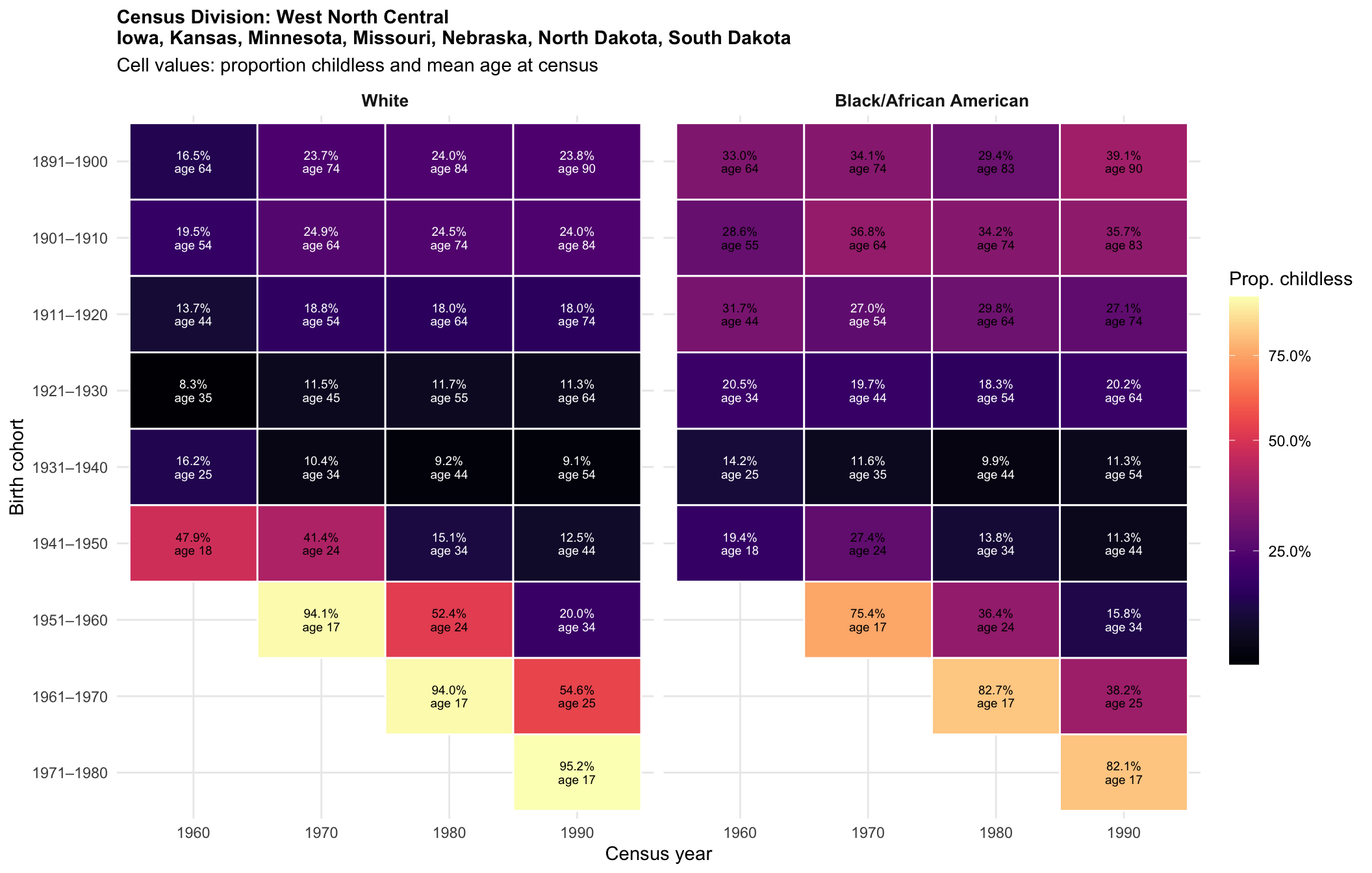
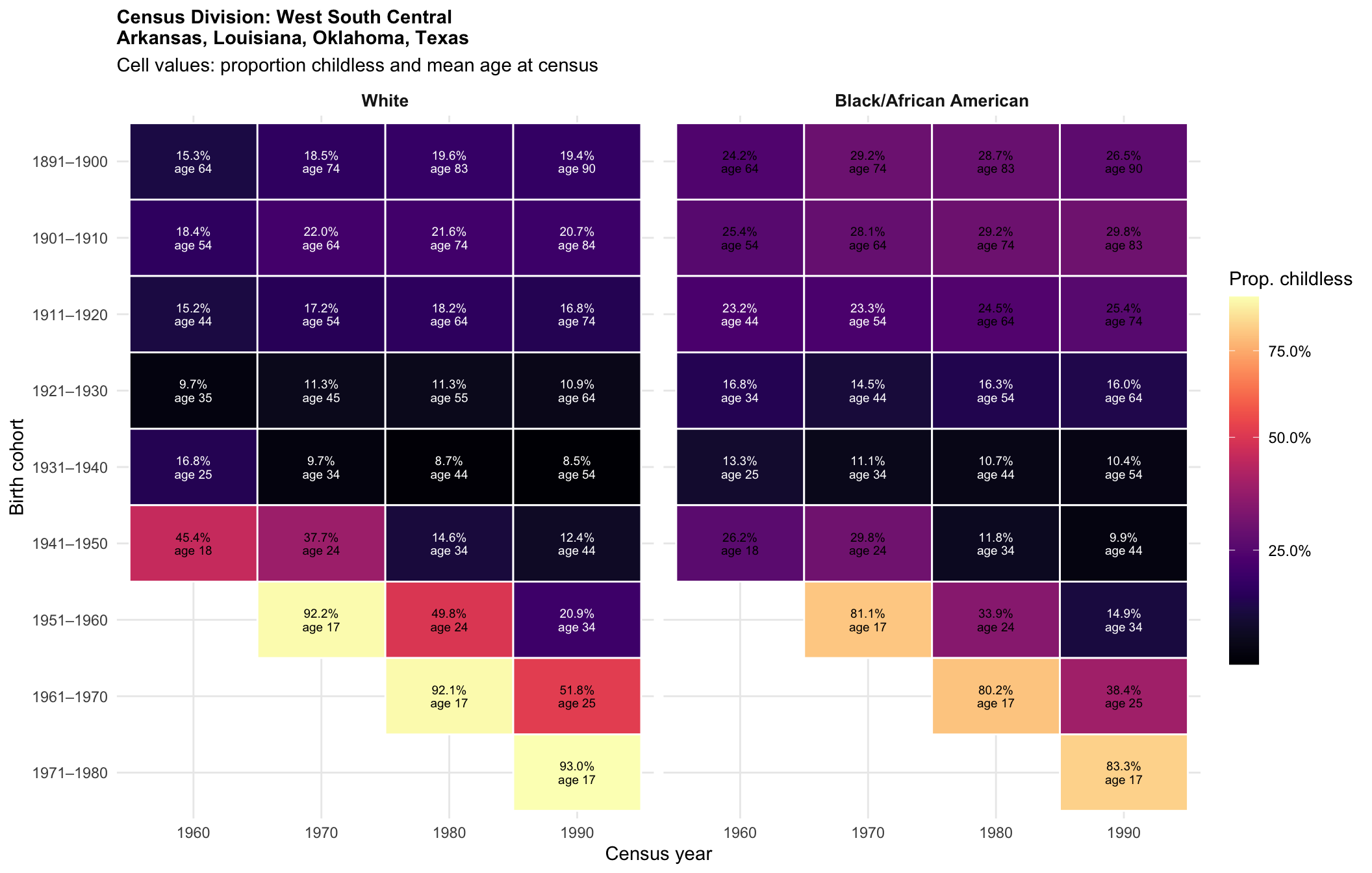
Version	Author	Date
5634d2b	Tina Lasisi	2026-04-16

Choropleth maps: Birth Cohort × Age Group (by division)

all_state_names <- sort(unique(data_cohort$state_name))

plot_cohort_grid_regional(
  cohort_division, "White",
  group_var    = "division",
  state_lookup = state_to_division,
  all_states   = all_state_names
)

Warning in left_join(., sub_reg %>% select(grp = all_of(group_var), prop_zero), : Detected an unexpected many-to-many relationship between `x` and `y`.
ℹ Row 1 of `x` matches multiple rows in `y`.
ℹ Row 11 of `y` matches multiple rows in `x`.
ℹ If a many-to-many relationship is expected, set `relationship =
  "many-to-many"` to silence this warning.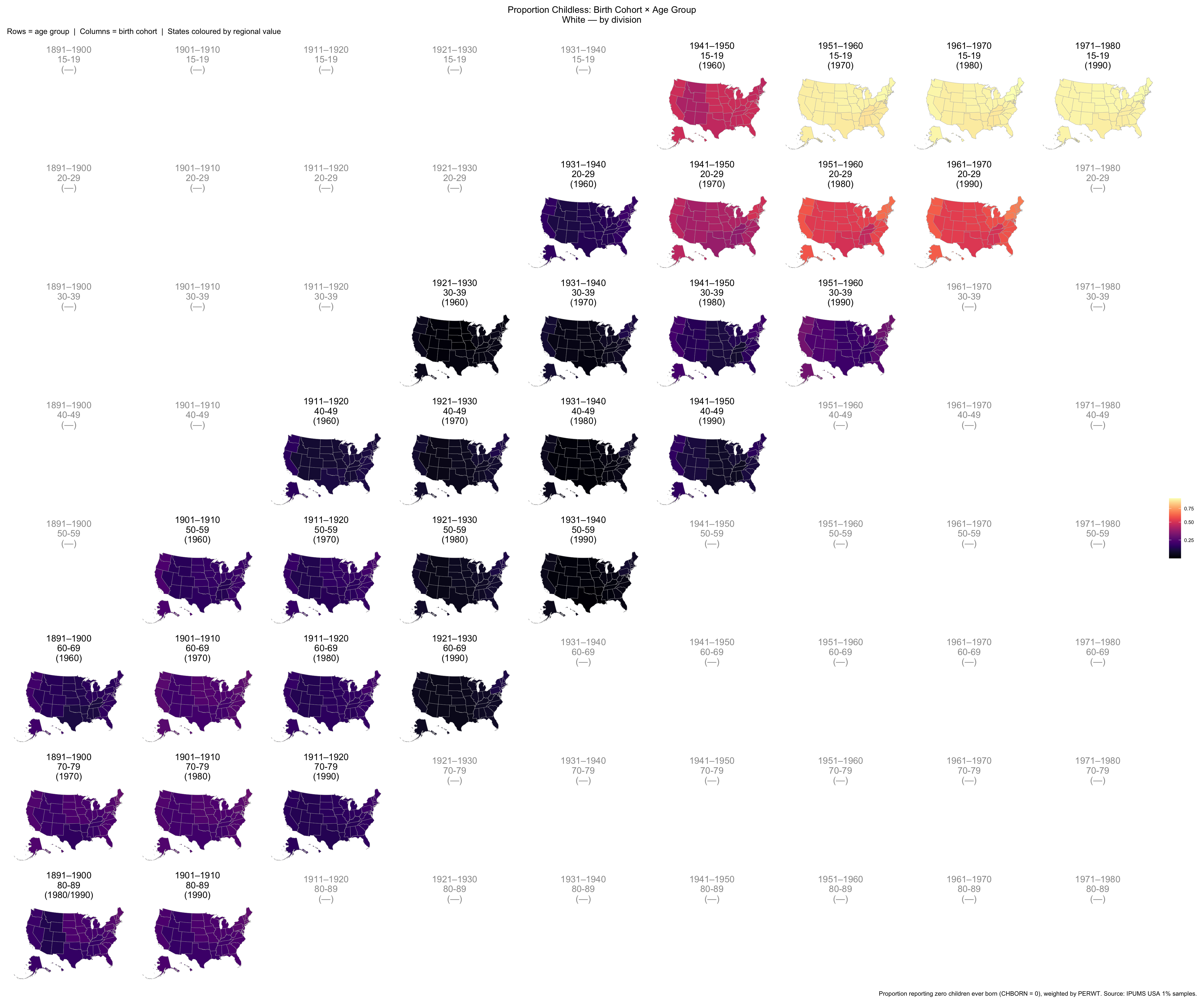

plot_cohort_grid_regional(
  cohort_division, "Black/African American",
  group_var    = "division",
  state_lookup = state_to_division,
  all_states   = all_state_names
)

Warning in left_join(., sub_reg %>% select(grp = all_of(group_var), prop_zero), : Detected an unexpected many-to-many relationship between `x` and `y`.
ℹ Row 1 of `x` matches multiple rows in `y`.
ℹ Row 11 of `y` matches multiple rows in `x`.
ℹ If a many-to-many relationship is expected, set `relationship =
  "many-to-many"` to silence this warning.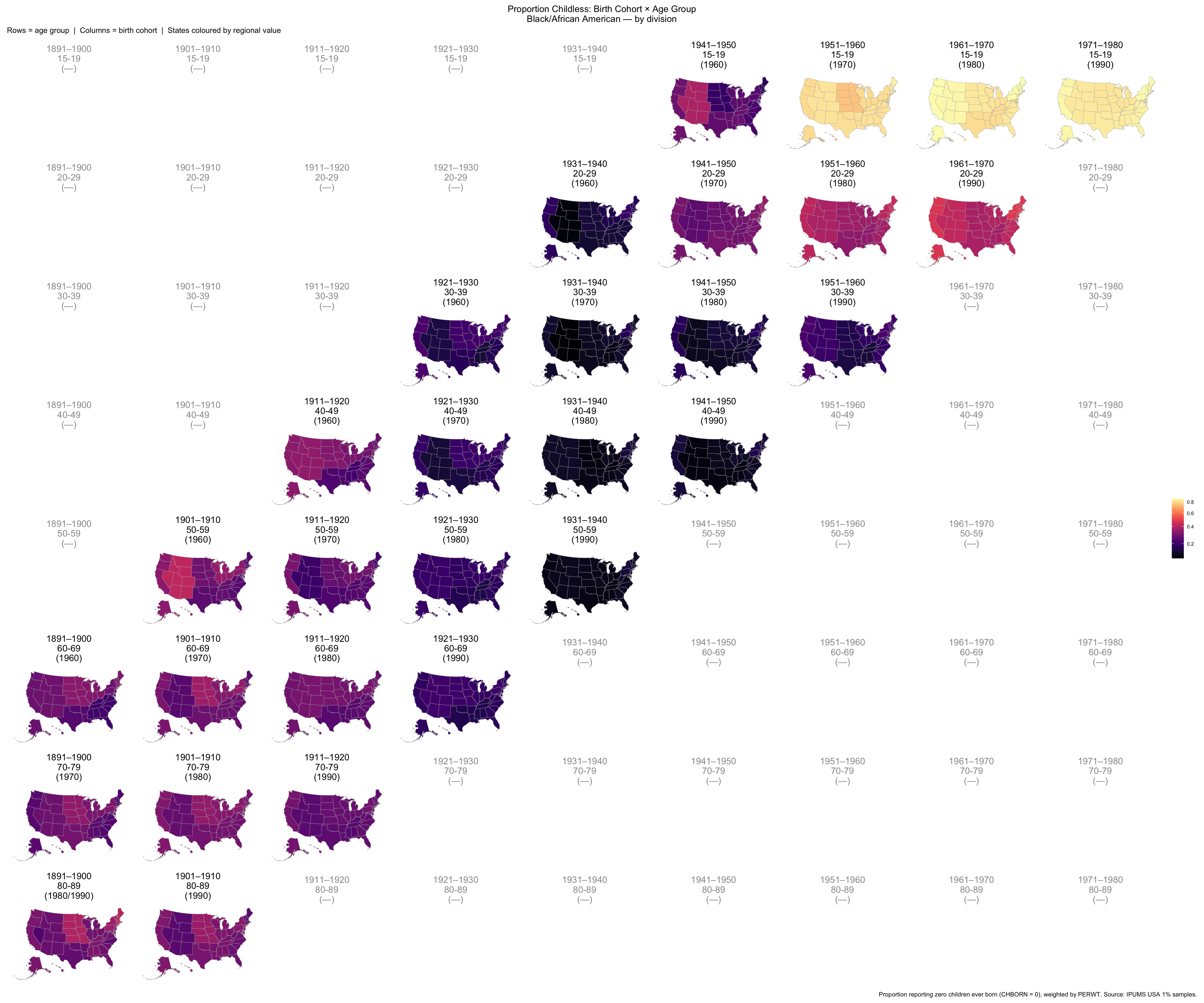

9d. Regional cohort trajectories: College sports conferences

cohort_conf <- data_cohort %>%
  mutate(conference = state_to_conference(as.character(STATEFIP))) %>%
  filter(!is.na(conference)) %>%
  group_by(conference, cohort_label, YEAR, AGE_RANGE, RACE) %>%
  summarise(
    n_obs     = n(),
    prop_zero = weighted.mean(chborn_num == 0, w = PERWT),
    n_pop     = sum(PERWT),
    mean_age  = weighted.mean(AGE, w = PERWT),
    .groups   = "drop"
  ) %>%
  mutate(
    prop_zero = prop_zero,
    age_label = paste0("age ", round(mean_age)),
    completed = AGE_RANGE >= "50-59"
  ) %>%
  filter(cohort_label %in% cohorts_of_interest)

Trajectory plots (per conference)

for (conf in sort(unique(cohort_conf$conference))) {
  conf_cohort <- cohort_conf %>%
    filter(conference == conf, !is.na(prop_zero))

  if (nrow(conf_cohort) == 0) next

  states_in_conf <- data_cohort %>%
    mutate(conference = state_to_conference(as.character(STATEFIP))) %>%
    filter(conference == conf) %>%
    pull(state_name) %>% unique() %>% sort()

  plot_title <- paste0("Conference: ", conf, "\n",
                       str_wrap(paste(states_in_conf, collapse = ", "), width = 80))

  p <- plot_cohort_stability(conf_cohort, title = plot_title)

  print(p)
  cat("\n\n")
}

Past versions of cohort-conference-plots-1.png

Version	Author	Date
5634d2b	Tina Lasisi	2026-04-16
027da76	Tina Lasisi	2026-04-14
71cf78a	Tina Lasisi	2026-04-14
34bd822	Tina Lasisi	2026-04-14
9d44b29	Tina Lasisi	2026-04-14

Past versions of cohort-conference-plots-2.png

Version	Author	Date
5634d2b	Tina Lasisi	2026-04-16
027da76	Tina Lasisi	2026-04-14
71cf78a	Tina Lasisi	2026-04-14
34bd822	Tina Lasisi	2026-04-14
9d44b29	Tina Lasisi	2026-04-14

Past versions of cohort-conference-plots-3.png

Version	Author	Date
5634d2b	Tina Lasisi	2026-04-16
027da76	Tina Lasisi	2026-04-14
71cf78a	Tina Lasisi	2026-04-14
34bd822	Tina Lasisi	2026-04-14
9d44b29	Tina Lasisi	2026-04-14

Past versions of cohort-conference-plots-4.png

Version	Author	Date
5634d2b	Tina Lasisi	2026-04-16
027da76	Tina Lasisi	2026-04-14
71cf78a	Tina Lasisi	2026-04-14
34bd822	Tina Lasisi	2026-04-14
9d44b29	Tina Lasisi	2026-04-14

Past versions of cohort-conference-plots-5.png

Version	Author	Date
5634d2b	Tina Lasisi	2026-04-16
027da76	Tina Lasisi	2026-04-14
71cf78a	Tina Lasisi	2026-04-14
34bd822	Tina Lasisi	2026-04-14
9d44b29	Tina Lasisi	2026-04-14

Cohort × Census Year matrices (per conference)

for (conf in sort(unique(cohort_conf$conference))) {
  conf_mat <- cohort_conf %>%
    filter(conference == conf)

  if (nrow(conf_mat) == 0) next

  states_in_conf <- data_cohort %>%
    mutate(conference = state_to_conference(as.character(STATEFIP))) %>%
    filter(conference == conf) %>%
    pull(state_name) %>% unique() %>% sort()

  mat_title <- paste0("Conference: ", conf, "\n",
                      str_wrap(paste(states_in_conf, collapse = ", "), width = 80))

  p <- plot_cohort_matrix(conf_mat, title = mat_title)
  print(p)
  cat("\n\n")
}

Past versions of cohort-conference-matrix-1.png

Version	Author	Date
5634d2b	Tina Lasisi	2026-04-16

Past versions of cohort-conference-matrix-2.png

Version	Author	Date
5634d2b	Tina Lasisi	2026-04-16

Past versions of cohort-conference-matrix-3.png

Version	Author	Date
5634d2b	Tina Lasisi	2026-04-16

Past versions of cohort-conference-matrix-4.png

Version	Author	Date
5634d2b	Tina Lasisi	2026-04-16

Past versions of cohort-conference-matrix-5.png

Version	Author	Date
5634d2b	Tina Lasisi	2026-04-16

Choropleth maps: Birth Cohort × Age Group (by conference)

plot_cohort_grid_regional(
  cohort_conf, "White",
  group_var    = "conference",
  state_lookup = state_to_conference,
  all_states   = all_state_names
)

Warning in left_join(., sub_reg %>% select(grp = all_of(group_var), prop_zero), : Detected an unexpected many-to-many relationship between `x` and `y`.
ℹ Row 1 of `x` matches multiple rows in `y`.
ℹ Row 9 of `y` matches multiple rows in `x`.
ℹ If a many-to-many relationship is expected, set `relationship =
  "many-to-many"` to silence this warning.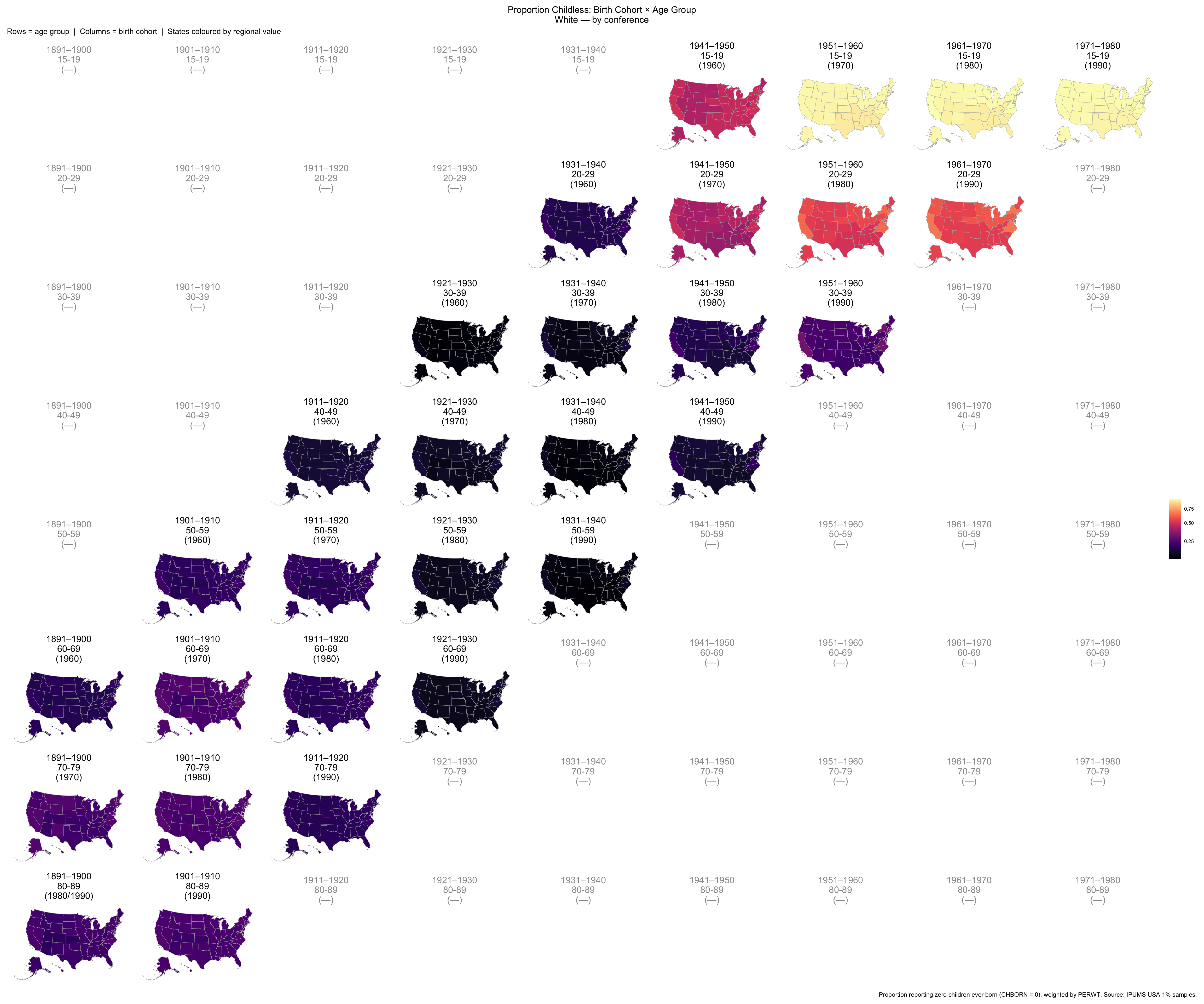

plot_cohort_grid_regional(
  cohort_conf, "Black/African American",
  group_var    = "conference",
  state_lookup = state_to_conference,
  all_states   = all_state_names
)

Warning in left_join(., sub_reg %>% select(grp = all_of(group_var), prop_zero), : Detected an unexpected many-to-many relationship between `x` and `y`.
ℹ Row 1 of `x` matches multiple rows in `y`.
ℹ Row 9 of `y` matches multiple rows in `x`.
ℹ If a many-to-many relationship is expected, set `relationship =
  "many-to-many"` to silence this warning.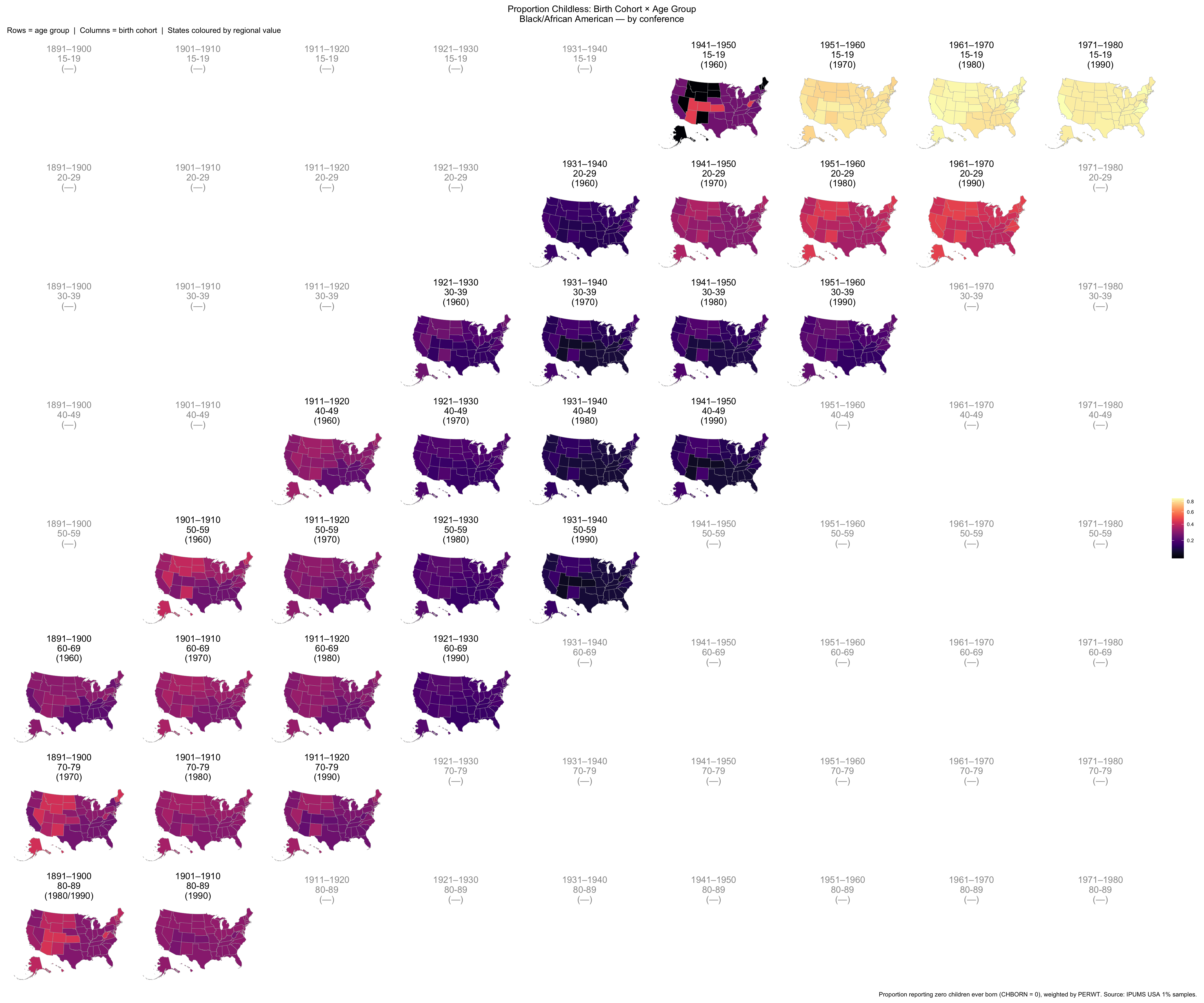

Session info

sessionInfo()

R version 4.5.3 (2026-03-11)
Platform: aarch64-apple-darwin20
Running under: macOS Tahoe 26.4.1

Matrix products: default
BLAS:   /Library/Frameworks/R.framework/Versions/4.5-arm64/Resources/lib/libRblas.0.dylib 
LAPACK: /Library/Frameworks/R.framework/Versions/4.5-arm64/Resources/lib/libRlapack.dylib;  LAPACK version 3.12.1

locale:
[1] C.UTF-8/C.UTF-8/C.UTF-8/C/C.UTF-8/C.UTF-8

time zone: America/Detroit
tzcode source: internal

attached base packages:
[1] stats     graphics  grDevices utils     datasets  methods   base     

other attached packages:
 [1] ggrepel_0.9.8     scales_1.4.0      patchwork_1.3.1   viridis_0.6.5    
 [5] viridisLite_0.4.2 usmap_1.0.0       data.table_1.17.6 lubridate_1.9.4  
 [9] forcats_1.0.0     stringr_1.6.0     dplyr_1.1.4       purrr_1.2.0      
[13] readr_2.1.5       tidyr_1.3.1       tibble_3.3.0      ggplot2_3.5.2    
[17] tidyverse_2.0.0   ipumsr_0.10.0     workflowr_1.7.1  

loaded via a namespace (and not attached):
 [1] gtable_0.3.6       xfun_0.54          bslib_0.9.0        processx_3.8.6    
 [5] callr_3.7.6        tzdb_0.5.0         vctrs_0.6.5        tools_4.5.3       
 [9] ps_1.9.1           generics_0.1.4     proxy_0.4-27       pkgconfig_2.0.3   
[13] KernSmooth_2.23-26 RColorBrewer_1.1-3 S7_0.2.1           lifecycle_1.0.4   
[17] compiler_4.5.3     farver_2.1.2       git2r_0.36.2       getPass_0.2-4     
[21] codetools_0.2-20   hipread_0.2.6      httpuv_1.6.16      class_7.3-23      
[25] htmltools_0.5.8.1  sass_0.4.10        yaml_2.3.10        later_1.4.2       
[29] pillar_1.11.1      jquerylib_0.1.4    whisker_0.4.1      classInt_0.4-11   
[33] cachem_1.1.0       tidyselect_1.2.1   digest_0.6.37      stringi_1.8.7     
[37] sf_1.0-21          labeling_0.4.3     rprojroot_2.1.1    fastmap_1.2.0     
[41] grid_4.5.3         cli_3.6.5          magrittr_2.0.4     utf8_1.2.6        
[45] dichromat_2.0-0.1  e1071_1.7-16       withr_3.0.2        promises_1.3.3    
[49] timechange_0.3.0   rmarkdown_2.29     httr_1.4.7         gridExtra_2.3     
[53] hms_1.1.3          evaluate_1.0.4     knitr_1.50         haven_2.5.5       
[57] rlang_1.1.6        Rcpp_1.1.0         zeallot_0.2.0      DBI_1.2.3         
[61] glue_1.8.0         xml2_1.3.8         usmapdata_1.0.0    rstudioapi_0.17.1 
[65] jsonlite_2.0.0     R6_2.6.1           units_1.0-0        fs_1.6.6          

Session information

sessionInfo()

R version 4.5.3 (2026-03-11)
Platform: aarch64-apple-darwin20
Running under: macOS Tahoe 26.4.1

Matrix products: default
BLAS:   /Library/Frameworks/R.framework/Versions/4.5-arm64/Resources/lib/libRblas.0.dylib 
LAPACK: /Library/Frameworks/R.framework/Versions/4.5-arm64/Resources/lib/libRlapack.dylib;  LAPACK version 3.12.1

locale:
[1] C.UTF-8/C.UTF-8/C.UTF-8/C/C.UTF-8/C.UTF-8

time zone: America/Detroit
tzcode source: internal

attached base packages:
[1] stats     graphics  grDevices utils     datasets  methods   base     

other attached packages:
 [1] ggrepel_0.9.8     scales_1.4.0      patchwork_1.3.1   viridis_0.6.5    
 [5] viridisLite_0.4.2 usmap_1.0.0       data.table_1.17.6 lubridate_1.9.4  
 [9] forcats_1.0.0     stringr_1.6.0     dplyr_1.1.4       purrr_1.2.0      
[13] readr_2.1.5       tidyr_1.3.1       tibble_3.3.0      ggplot2_3.5.2    
[17] tidyverse_2.0.0   ipumsr_0.10.0     workflowr_1.7.1  

loaded via a namespace (and not attached):
 [1] gtable_0.3.6       xfun_0.54          bslib_0.9.0        processx_3.8.6    
 [5] callr_3.7.6        tzdb_0.5.0         vctrs_0.6.5        tools_4.5.3       
 [9] ps_1.9.1           generics_0.1.4     proxy_0.4-27       pkgconfig_2.0.3   
[13] KernSmooth_2.23-26 RColorBrewer_1.1-3 S7_0.2.1           lifecycle_1.0.4   
[17] compiler_4.5.3     farver_2.1.2       git2r_0.36.2       getPass_0.2-4     
[21] codetools_0.2-20   hipread_0.2.6      httpuv_1.6.16      class_7.3-23      
[25] htmltools_0.5.8.1  sass_0.4.10        yaml_2.3.10        later_1.4.2       
[29] pillar_1.11.1      jquerylib_0.1.4    whisker_0.4.1      classInt_0.4-11   
[33] cachem_1.1.0       tidyselect_1.2.1   digest_0.6.37      stringi_1.8.7     
[37] sf_1.0-21          labeling_0.4.3     rprojroot_2.1.1    fastmap_1.2.0     
[41] grid_4.5.3         cli_3.6.5          magrittr_2.0.4     utf8_1.2.6        
[45] dichromat_2.0-0.1  e1071_1.7-16       withr_3.0.2        promises_1.3.3    
[49] timechange_0.3.0   rmarkdown_2.29     httr_1.4.7         gridExtra_2.3     
[53] hms_1.1.3          evaluate_1.0.4     knitr_1.50         haven_2.5.5       
[57] rlang_1.1.6        Rcpp_1.1.0         zeallot_0.2.0      DBI_1.2.3         
[61] glue_1.8.0         xml2_1.3.8         usmapdata_1.0.0    rstudioapi_0.17.1 
[65] jsonlite_2.0.0     R6_2.6.1           units_1.0-0        fs_1.6.6